Big O Notation (OCR A Level Computer Science)

Big O Notation

What is Big O Notation?

• Big O Notation is used to express the complexity of an algorithm

• Describes the scalability of an algorithm as it's order (O), referred to in Computer Science as Big O Notation

• Named after the German mathematician Edmund Landau 

• Has two simple rules

  • Remove all terms except the one with the largest factor or exponent

  • Remove any constants

• There are several classifications used in Big O Notation, ranging from fast and efficient to slow and inefficient. These are all covered below

Constant

• O(1), read as Big-O One, describes an algorithm that takes constant time, that is, requires the same number of instructions to be executed, regardless of the size of the input data

• For example, to calculate the length of a string ‘s’ the following code could be used:

  • totalLength = len(s)

• No matter how long the string is, it will always take the same number of instructions to find the length

Linear

• O(n), read as Big-O n, describes an algorithm that takes linear time, that is, as the input size increases, the number of instructions to be executed grows proportionally

• For example, a linear search of 1000 items will take 10 times longer to search than an array of 100 items

• Implementing linear time requires use of iteration i.e. for loops and while loops

• In the example of sumNumbers1, a basic (for i = 1 to n) loop is used

• Below is an example of an algorithm that uses multiple for loops

function loop

x = input
for i = 1 to x
	print(x)
next i

a = 0
for j = 1 to x
	a = a + 1
next j
print(a)

b = 1
for k = 1 to x
	b = b + 1
next k
print(b)

endfunction

• When the user inputs a value of x, each loop will run x times, performing varied instructions in each loop

• The total number of instructions executed in this algorithm are as follows:

  • +1 for (x = input)

  • +x for the first for loop

  • +1 for (a = 0)

  • +x for the second for loop

  • +1 for (output a)

  • +1 for (b =1)

  • +x for the third for loop

  • +1 for (output b)

• The total number of instructions executed would therefore be: 3x + 5

• As x increases the total number of instructions executed also increases as shown in the table below

Linear Time: Number of Instructions Executed

• The constant term (5) contributes less and less to the overall time complexity as x increases. 3x is the significant contributing term and causes the overall time complexity to grow linearly in a straight line as x increases

Polynomial

• O(n²), read as Big-O n-squared, describes an algorithm that takes squared time to complete. This means the performance is proportional to the square of the number of data inputs

• For example, a bubble sort is a polynomial time complexity algorithm. n passes are made, and for each pass n comparisons are made hence n*n or O(n²)

• Implementing polynomial time requires the use of nested iteration i.e. for loops or while loops, where each loop executes n times

• An example of a polynomial algorithm is shown below:

function timesTable

x = 12
for i = 1 to x
	for j = 1 to x
		print(i, “ x “, j, “ = “, i*j)
	next j
next i

for k = 1 to x
	print(k)
next k
print(“Hello World!”)

endfunction

• The above algorithm outputs the times tables from the 1 times table to the 12 times table. An arbitrary for loop (for k = 1 to 10) and output (print(“Hello World!”)) has been added for demonstration purposes as shown below

• The total number of instructions executed by this algorithm are as follows:

  • +1 for (x = 12)

  • +x * x for the nested for loop

  • +x for the non-nested for loop

  • +1 for (print(“Hello World!”))

• The total number of instructions executed would therefore be: x*x + x + 2 or, x² + x + 2

• As x increases the total number of instructions executed also increases as shown in the table below

Polynomial Time: Number of Instructions Executed

• The constant term (2) and linear term (x) contribute very little as x increases, making x² the significant contributing term

  • To put this algorithm into perspective, assuming it took one second per instruction, printing up to the 1,000,000 times table would take roughly 32,000 years

• Loops can be nested any number of times. In the example above, there are two loops nested. Each loop nested increases the polynomial time as shown below. Regardless of the number of loops nested, all are still referred to as polynomial time!

Big-O of Nested Loops

• Below is an example of a six nested algorithm. Note that the algorithm does nothing useful except demonstrate this nesting

for a = 1 to n
	for b = 1 to n
		for c = 1 to n
			for d = 1 to n
				for e = 1 to n
					for f = 1 to n
					next f
				next e
			next d
		next c
	next b
next a

Exponential

• Exponential time, read as Big-O 2-to-the-n, describes an algorithm that takes double the time to execute for each additional data input value. The number of instructions executed becomes very large, very quickly for each input value

• Few everyday algorithms use exponential time due to its sheer inefficiency. Some problems however can only be solved in exponential time

Exponential time: Number of Instructions Executed

Logarithmic

• Logarithmic time, read as Big-O log-n, describes an algorithm that takes very little time as the size of the input grows larger

• Logarithmic time in computer science is usually measured in base 2. A logarithm is the value the base must be raised to to equal another number, for example:

  • 2³ = 8, log₂(8) = 3, i.e. to get to the value 8, 2 must be raised to the power of 3

• A binary search is an example of logarithmic time complexity. Doubling the size of the input data has very little effect on the overall number of instructions executed by the algorithm, as shown below:

Logarithmic Time: Number of Instructions Executed

• As shown above, increasing the number of input values to over one billion did very little to the number of instructions taken to complete the algorithm

Comparison of Complexity

• All algorithms have a best case, average case and worst case complexities.

• These are defined as the best possible outcome, the average outcome and the worst possible outcome in terms of the number of instructions required to complete the algorithm

• Best case complexity is where the algorithm performs most efficiently such as a linear search or binary search finding the correct item on the first element O(1), or a bubble sort being supplied with an already sorted list O(n). A bubble sort must always make at least one pass, hence O(n)

• Average case complexity is where the algorithm performs neither at its best or worst on any given data. A linear search may find the item in the middle of the list and therefore have a Big-O notation of O(ⁿ/2), or a bubble sort sorting only half a list O(n² / 2)

• Worst case complexity is where an algorithm is at its least efficient such as a linear search finding the item in the last position, or not at all O(n), or a bubble sort sorting a reversed list O(ⁿ2), i.e. a list whose items are ordered highest to lowest

• Big-O notation is almost always measured by the worst case performance of an algorithm. This allows programmers to accurately select appropriate algorithms for problems and have a guaranteed minimum performance level

• The graphical representation of constant, linear, polynomial, exponential and logarithmic times is shown below

Big-O Time Complexity Graph

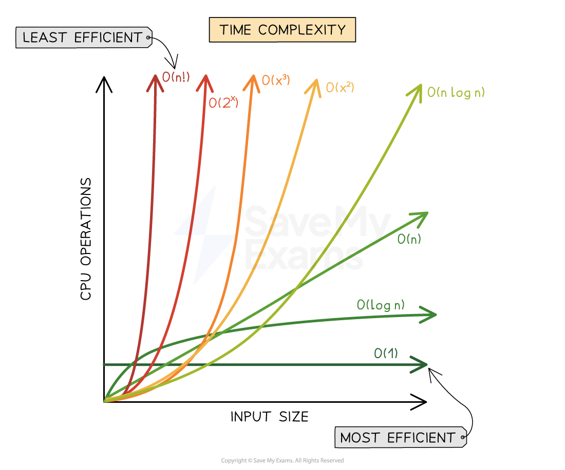
Figure 1: Graph of Time Complexity for Big-O Notation Functions

• From the graph, exponential time (2ⁿ) grows the quickest and therefore is the most inefficient form of algorithm, followed by polynomial time (n²), linear time (n), logarithmic time (logn) and finally constant time (1)

• Further time complexities exist such as factorial time (n!) which performs worse than exponential time and linear-logarithmic time (nlogn) which sits between polynomial and linear time. Merge sort is an example of an algorithm that uses O(nlogn) time complexity

• The Big-O time complexity of an algorithm can be derived by inspecting its component parts

• It is important to know that when determining an algorithm's Big-O that only the dominant factor is used.

• This means the time complexity that contributes the most to the algorithm is used to describe the algorithm. For example:

  • 3x² + 4x + 5, which describes three nested loops, four standard loops and five statements is described as O(n²)

  • x² is the dominating factor. As the input size grows x² contributes proportionally more than the other factors

  • Coefficients are also removed from the Big-O notation. The 3 in 3x² acts as a multiplicative value whose contribution becomes smaller and smaller as the size of the input increases.

    • For an arbitrarily large value such as 10¹⁰⁰, which is 10 with one hundred 0’s after it, multiplying this number by 3 will have little contribution to the overall time complexity. 3 is therefore dropped from the overall time complexity

• The simplest way of deriving time complexity is to count the number of loops and nested loops in an algorithm.

function sumNumbers1(n)
	sum = 0
	for i = 1 to n
		sum = sum + n
	next i
	return sum
endfunction

• In the example above for sumNumbers1, a single for loop is present. As loops are O(n) and single statements are O(1), the overall Big-O notation is O(n), linear time, as the loop dominates constant time

function sumNumbers2(n)
	sum = n * (n+1)/2
	return sum
endfunction

• In the example above for sumNumbers2, a single statement is present with no loops. Statements are O(1) therefore making the overall Big-O notation O(1), constant time

function loop

x = input
for i = 1 to x
	print(x)
next i

a = 0
for j = 1 to x
	a = a + 1
next j
print(a)

b = 1
for k = 1 to x
	b = b + 1
next k
print(b)

endfunction

• In the example above for function loop, there are three loops present 3*O(n) and five statements 5*O(1). As the input size grows, the quantity of loops or statements becomes negligible, meaning coefficients eventually become factored out or removed. This leaves O(n) and O(1). As O(n) dominates O(1), the overall Big-O notation of this algorithm becomes O(n), linear time

function timesTable

x = 12
for i = 1 to x
	for j = 1 to x
		print(i, “ x “, j, “ = “, i*j)
	next j
next i

for k = 1 to x
	print(k)
next k
print(“Hello World!”)

endfunction

• In the example above for function timesTable, there is a single nesting of two loops O(n²), a single loop O(n) and a single statement O(1). As polynomial time dominates linear and constant time and that no coefficients are involved, the overall Big-O notation is O(n²)