The Normal Distribution (DP IB Applications & Interpretation (AI)): Revision Note

Properties of normal distribution

The binomial distribution is an example of a discrete probability distribution. The normal distribution is an example of a continuous probability distribution.

What is a continuous random variable?

• A continuous random variable (often abbreviated to CRV) is a random variable that can take any value within a range of infinitely many values

  • Continuous random variables usually measure something

  • For example, height, weight, time, etc

What is a continuous probability distribution?

• A continuous probability distribution is a probability distribution in which the random variable is continuous

• The probability of being a particular value is always zero

  • for any value k

• Instead we define the probability density function  for a specific value

  • This is a function that describes the relative likelihood that the random variable would be close to that value

  • We talk about the probability of  being within a certain range

• A continuous probability distribution can be represented by a continuous graph of its probability density function

  • The values for are along the horizontal axis, and probability density on the vertical axis

• The area under the graph between the points and is equal to 

  • The total area under the graph equals 1

• As for any value k, it does not matter if we use strict or weak inequalities

  • for any value k when X is a continuous random variable

What is a normal distribution? 

• A normal distribution is a type of continuous probability distribution

• The continuous random variable can follow a normal distribution if:

  • The distribution is symmetrical

  • The distribution is bell-shaped

• If follows a normal distribution then it is denoted 

  • means "is distributed as" or "has the distribution"

  • indicates the normal distribution

  • μ is the mean

  • σ² is the variance

    • σ is the standard deviation

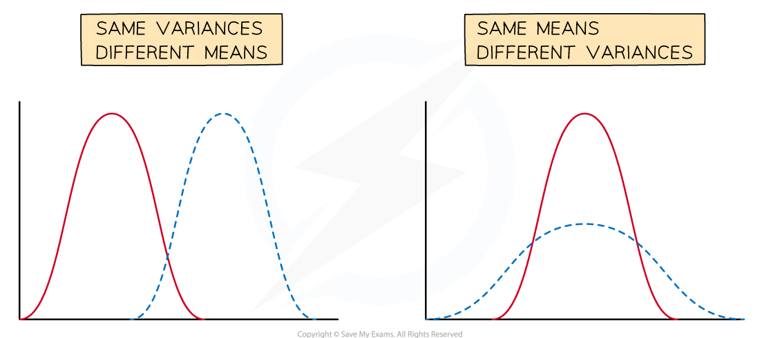
• If the mean changes then the graph is translated horizontally

• If the variance increases then the graph is widened horizontally and made shorter vertically to maintain the same area

  • A small variance leads to a tall curve with a narrow centre

  • A large variance leads to a short curve with a wide centre

What are the important properties of a normal distribution? 

• The mean is μ

• The variance is σ²

  • If you need the standard deviation remember to take the square root of this

• The normal distribution is symmetrical about  

  • Mean = Median = Mode = μ

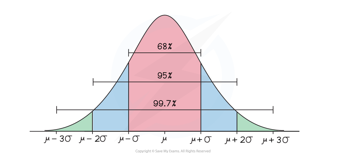
• You should be familiar with these results:

  • Approximately two-thirds (68%) of the data lies within one standard deviation of the mean (μ ± σ)

  • Approximately 95% of the data lies within two standard deviations of the mean (μ ± 2σ)

  • Nearly all of the data (99.7%) lies within three standard deviations of the mean (μ ± 3σ)

Modelling with normal distribution

What can be modelled using a normal distribution? 

• A lot of real-life continuous variables can be modelled by a normal distribution

  • provided that the population is large enough

  • and that the variable is symmetrical with one mode

• For a normal distribution  can take any real value

  • However values far from the mean (more than 4 standard deviations away from the mean) have a probability density of practically zero

  • This fact allows us to model variables that are not defined for all real values such as height and weight

What cannot be modelled using a normal distribution? 

• Variables which have more than one mode or no mode

  • For example: the number given by a random number generator

• Variables which are not symmetrical

  • For example: how long a human lives for