Experimental Design & Analysis (College Board AP® Physics 1: Algebra-Based): Exam Questions

1 hour6 questions
1a
Sme Calculator
2 marks
Diagram of a transformer with a coil, labelled pins A, B, C, and a plate on the right. Arrows are pointing to the pin and plate from outside.

Figure 1

A group of students are given a projectile launcher which consists of a spring with an attached plate, as shown in Figure 1. When the spring is compressed, the plate can be held in place by a pin at any of three positions A, B, or C.

The same spring diagram as figure 1, but a sphere is now compressing the spring to pin position C

Figure 2

Figure 2 shows a steel sphere placed against the plate, which is held in place by a pin at position C. The sphere is launched upon release of the pin.

The students have access to the projectile launcher and equipment usually found in a school laboratory.

The students are asked to take measurements to create a graph that could be used to determine the spring constant of the spring.

Describe an experimental procedure the students could use to collect the data needed to determine the spring constant of the spring. Include any steps necessary to reduce experimental uncertainty. If needed, you may include a simple diagram of the setup with your procedure.

1b
Sme Calculator
2 marks

Describe how the data collected in part a) could be plotted to create a linear graph, and how that graph would be analyzed to determine the spring constant k of the spring.

1c
Sme Calculator
1 mark

The students perform another experiment using the projectile launcher, where they measure the range of spheres of different masses and their time of flight. The spring constant of the spring is 6 space straight N divided by straight m. The following table shows the horizontal range R of each sphere and its time of flight t. The students create a graph with k open parentheses increment x close parentheses squared plotted on the vertical axis.

Compression distance (m)

Time of flight (s)

Range (m)

(A) 0.02

1.02

0.108

(B) 0.04

0.98

0.215

(C) 0.06

1.05

0.343

Table 1

Indicate which measured or calculated quantity could be plotted on the horizontal axis to yield a linear graph whose slope can be used to calculate an experimental value for the mass of the new sphere. You may use the remaining columns in the table above, as needed, to record any quantities (including units) that are not already in the table.

  • Vertical axis = k open parentheses increment x close parentheses squared

  • Horizontal axis = ........

1d
Sme Calculator
3 marks

i) On the grid in Figure 3, plot the appropriate quantities to determine the mass of the sphere. Clearly scale and label all axes, including units, as appropriate.
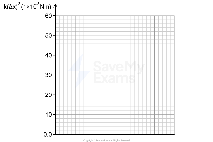
Blank graph with y-axis labelled "k(Δx)² (1×10⁻³ Nm)" ranging from 0 to 60, grid lines displayed.

Figure 3

ii) Draw a best fit line to the data graphed in part i).

1e
Sme Calculator
2 marks

Calculate an experimental value for the mass of the ball bearing using the best-fit line that you drew in Figure 3 in part ii).

Did this page help you?

2a
Sme Calculator
2 marks
Cylindrical container is half-filled with liquid. The container rests on a table.

Figure 1

A group of students are given a cylindrical container half filled with a liquid of unknown density rho. The students have access to an additional container with more of the same liquid, meter sticks, and a pressure sensor. They do not have access to a scale.

The students are asked to take measurements to create a graph that could be used to determine the density of the liquid. Describe an experimental procedure the students could use to collect the data needed to determine the density of the liquid. Include any steps necessary to reduce experimental uncertainty. If needed, you may include a simple diagram of the setup with your procedure.

2b
Sme Calculator
2 marks

Describe how the data collected in part a) could be plotted to create a linear graph and how that graph would be analyzed to determine the density rho of the liquid.

2c
Sme Calculator
4 marks
Diagram showing water flowing horizontally from a tank on a table, with height marked as "h" and initial velocity marked as "v₀" as it exits.

Figure 2

Students perform an experiment with a cylinder which is filled with water, as shown in Figure 2. The students make a small hole in the side of the cylinder and measure the speed v at which water exits the hole. The students plug the first hole, make another one at a different height, and repeat this procedure. Table 1 shows the height h of each hole relative to the top of the water, and the corresponding water speed v.

Height, h (m)

Speed, v (m/s)

0.25

2.2

0.20

2.0

0.15

1.8

0.10

1.4

0.05

1.1

Table 1

The students correctly determine that the relationship between h and v is given by v space equals space square root of 2 g h end root . The students create a graph with v squared plotted on the vertical axis.

i) Indicate which measured or calculated quantity could be plotted on the horizontal axis to yield a linear graph whose slope can be used to calculate an experimental value for the acceleration due to gravity. Use the blank columns in the table to list any calculated quantities you will graph other than the data provided.

Vertical axis: bottom enclose space space space space space space space space space space space space space space space space space v squared space space space space space space space space space space space space space space space space space space space end enclose Horizontal axis: bottom enclose space space space space space space space space space space space space space space space space space space space space space space space space space space space space space space space space space space space space space space end enclose

ii) On the grid in Figure 3, plot the appropriate quantities to determine the acceleration due to gravity. Clearly scale and label all axes, including units, as appropriate.

A graph with a 6x6 grid of large squares. Each large square contains 5 small squares. The vertical axis runs from 0.0 to 6.0. It is labelled v^2 with units m^2/s^2.

Figure 3

iii) Draw a best fit line for the data graphed in part ii).

2d
Sme Calculator
2 marks

Calculate an experimental value for the acceleration due to gravity using the best-fit line that you drew in part c)iii).

Did this page help you?

3a
Sme Calculator
2 marks

A student is investigating the relationship between the length of a simple pendulum and its period of oscillation. The student has access to a stopwatch, a meter rule, a pendulum bob, a retort stand with a clamp, and a protractor.

Describe an experimental procedure the student could use to collect data to verify the relationship between the length of the pendulum and the period of oscillation. Include any steps necessary to reduce experimental uncertainty. If needed, you may include a simple diagram of the setup with your procedure.

3b
Sme Calculator
2 marks

Describe how the collected data should be plotted to create a linear graph, and how that graph would be analyzed to verify the relationship between length and period.

3c
Sme Calculator
6 marks

The experiment is now modified to investigate the forces acting on a mass moving in a vertical circle. The student releases a pendulum bob from a horizontal position and measures the tension in the string at the lowest point of the swing. The student also measures the velocity of the bob at this point. The recorded data is shown in table 1.

Velocity (v) (straight m divided by straight s)

Velocity Squared (v squared) (straight m squared divided by straight s squared)

Tension (T) (N)

1.0

1.0

4.0

1.5

2.25

6.0

2.0

4.0

8.0

2.5

6.25

10.0

3.0

9.0

12.0

Table 1

The relationship between tension, velocity, and the length of the string is given by:

T space minus space m g space equals space fraction numerator m v squared over denominator L end fraction

Where:

  • T is the tension in the string

  • m space equals space 0.15 space kg is the mass of the pendulum bob

  • v is the velocity at the lowest point

  • L is the length of the string,

  • g space equals space 10 space straight m divided by straight s squared

i) Indicate two quantities that when graphed produce a straight-line relationship that could be used to determine the length of the string.


ii) Plot on the grid in Figure 1 the data points for the quantities indicated in part i). Clearly scale and label all axes, including units.

Blank graph with grid lines; x-axis numbered 1-9, y-axis from 4-12. Watermarked with "Save My Exams" in the centre.

Figure 1


iii) Draw a best-fit line to the data graphed in part ii).


iv) Calculate an experimental value for the length of the string using the best-fit line that you drew in part iii).

Did this page help you?

4a
Sme Calculator
2 marks

A student has a rubber ball of known mass m which they release from rest from height h. The student is asked to verify the relationship between the impulse exerted on the ball upon impact with the ground and the change in its momentum. The student has access to a force sensor, a motion sensor, and other standard laboratory equipment.

Describe an experimental procedure the student could use to collect data that would allow them to verify the relationship between impulse and change in momentum. Include any steps necessary to reduce experimental uncertainty. If needed, you may include a simple diagram of the setup with your procedure.

4b
Sme Calculator
2 marks

Describe how the collected data should be analyzed to verify the relationship between impulse and change in momentum.

4c
Sme Calculator
4 marks

The experiment is repeated using a clay ball of mass 50 g which is dropped from different heights above the ground. The clay ball sticks to the force sensor on the ground upon impact. The student's measurements are shown in Table 1.

Drop height

h space open parentheses straight m close parentheses

Average
Impact Force

F subscript a v g end subscript space open parentheses straight N close parentheses

Impact Time

increment t space open parentheses straight s close parentheses

‎ ‎ ‎ ‎ ‎ ‎ ‎ ‎ ‎ ‎ ‎ ‎ ‎ ‎ ‎ ‎ ‎ ‎

‎ ‎ ‎ ‎ ‎ ‎ ‎ ‎ ‎ ‎ ‎ ‎ ‎ ‎ ‎ ‎ ‎ ‎

0.15

4.0

0.023

‎ ‎ ‎ ‎ ‎ ‎ ‎ ‎ ‎ ‎ ‎ ‎ ‎ ‎ ‎ ‎ ‎ ‎

‎ ‎ ‎ ‎ ‎ ‎ ‎ ‎ ‎ ‎ ‎ ‎ ‎ ‎ ‎ ‎ ‎ ‎

0.30

5.7

0.021

‎ ‎ ‎ ‎ ‎ ‎ ‎ ‎ ‎ ‎ ‎ ‎ ‎ ‎ ‎ ‎ ‎ ‎

‎ ‎ ‎ ‎ ‎ ‎ ‎ ‎ ‎ ‎ ‎ ‎ ‎ ‎ ‎ ‎ ‎ ‎

0.45

7.9

0.019

‎ ‎ ‎ ‎ ‎ ‎ ‎ ‎ ‎ ‎ ‎ ‎ ‎ ‎ ‎ ‎ ‎ ‎

‎ ‎ ‎ ‎ ‎ ‎ ‎ ‎ ‎ ‎ ‎ ‎ ‎ ‎ ‎ ‎ ‎ ‎

0.60

10.0

0.017

‎ ‎ ‎ ‎ ‎ ‎ ‎ ‎ ‎ ‎ ‎ ‎ ‎ ‎ ‎ ‎ ‎ ‎

‎ ‎ ‎ ‎ ‎ ‎ ‎ ‎ ‎ ‎ ‎ ‎ ‎ ‎ ‎ ‎ ‎ ‎

0.75

12.6

0.015

‎ ‎ ‎ ‎ ‎ ‎ ‎ ‎ ‎ ‎ ‎ ‎ ‎ ‎ ‎ ‎ ‎ ‎

‎ ‎ ‎ ‎ ‎ ‎ ‎ ‎ ‎ ‎ ‎ ‎ ‎ ‎ ‎ ‎ ‎ ‎

0.90

17.5

0.012

‎ ‎ ‎ ‎ ‎ ‎ ‎ ‎ ‎ ‎ ‎ ‎ ‎ ‎ ‎ ‎ ‎ ‎

‎ ‎ ‎ ‎ ‎ ‎ ‎ ‎ ‎ ‎ ‎ ‎ ‎ ‎ ‎ ‎ ‎ ‎

Table 1

i) Indicate two quantities that when graphed produce a straight line that could be used to calculate an experimental value for the acceleration due to gravity. You may use the blank columns in the table for any quantities you graph other than the given data. Use the blank columns in the table to list any calculated quantities (including units) you will graph other than the data provided.

Vertical Axis: ⎽⎽⎽⎽⎽⎽⎽⎽⎽⎽⎽⎽⎽⎽⎽⎽⎽⎽⎽⎽ ‎ ‎ ‎ ‎ ‎ ‎ ‎ ‎ ‎ Horizontal Axis: ⎽⎽⎽⎽⎽⎽⎽⎽⎽⎽⎽⎽⎽⎽⎽⎽⎽⎽⎽⎽

ii) Plot the data points for the quantities indicated in part c)i) on the following graph. Clearly scale and label all axes, including units.

Rectangular grid with small squares, divided into larger sections by thicker lines, resembling graph paper for mathematical or design purposes.

iii) Draw a best fit line to the data graphed in part c)(ii).

4d
Sme Calculator
2 marks

Calculate an experimental value for the acceleration due to gravity using the best-fit line that you drew in part c)iii).

Did this page help you?

5a
Sme Calculator
2 marks
Two carts with mass M. Cart 2 contains a plunger-spring system. Before recoil: carts at rest next to each other, spring compressed within Cart 2. After recoil: carts move apart, spring extended.

Figure 1

A group of students have two carts, Cart 1 and Cart 2, each of identical, unknown mass M. The carts are initially at rest and placed next to each other on a horizontal track. Cart 2 contains a compressed spring which can be released by pressing a switch on top of the cart. When the switch is pressed, the spring expands and pushes a plunger outward, causing the two carts to recoil, as shown in Figure 1. Blocks of different known masses can be attached to each cart.

The group of students is asked to determine whether the total momentum of the system is conserved. The students have access to equipment that can be found in a typical school physics laboratory.

Describe an experimental procedure the students could use to collect the data needed to determine whether the total momentum of the system is conserved. Provide enough detail so that the experiment could be replicated, including any steps necessary to reduce experimental uncertainty.

5b
Sme Calculator
2 marks

Describe how the data collected in part a) could be graphed and how that graph would be analyzed to determine whether the total momentum of the system is conserved.

5c4 marks
Two carts, 1 and 2, of mass M on a track. Cart 2, with a spring and a block on top, is against a wall to the left. Cart 1 is to the right of Cart 2, with 4 blocks on top.

Figure 2

In a later experiment, Cart 2 is placed next to a wall. When the switch is pressed, the spring expands and the plunger pushes on the wall, causing Cart 2 to move towards Cart 1, as shown in Figure 2. Cart 1 is initially at rest. After the collision, the two carts stick together and move along the track with speed v. Blocks of identical, known mass can be attached to Cart 1 and Cart 2, as long as the total mass of the system remains constant. The spring constant k of the spring in Cart 2 is unknown. When the spring is contained within the cart, it is compressed by a fixed distance x from its equilibrium position.

The students are asked to determine the value of the spring constant of the spring. The students measure the combined mass M subscript 1 comma B end subscript of Cart 1 and the blocks, the combined mass M subscript 2 comma B end subscript of Cart 2 and the blocks, and the final speed of the two-cart-block system.

The students measure the fixed value x space equals space 0.062 space straight m. The students repeat the experiment using different numbers of blocks on each cart and collect the data shown in the following table.

Combined mass of Cart 1 and blocks,

M subscript 1 comma B end subscript space open parentheses kg close parentheses

Combined mass of Cart 2 and blocks,

M subscript 2 comma B end subscript space open parentheses kg close parentheses

Final speed of the two-cart-block system,

v space open parentheses straight m divided by straight s close parentheses

‎ ‎ ‎ ‎ ‎ ‎ ‎ ‎ ‎ ‎ ‎ ‎ ‎ ‎ ‎ ‎ ‎ ‎ ‎ ‎ ‎ ‎ ‎ ‎ ‎ ‎ ‎ ‎ ‎ ‎ ‎ ‎ ‎ ‎ ‎ ‎ ‎ ‎ ‎ ‎ ‎ ‎ ‎ ‎ ‎ ‎ ‎ ‎ ‎ ‎ ‎ ‎ ‎ ‎ ‎ ‎ ‎ ‎ ‎ ‎ ‎ ‎ ‎ ‎ ‎ ‎ ‎ ‎ ‎ ‎ ‎ ‎ ‎ ‎ ‎ ‎ ‎ ‎ ‎ ‎ ‎ ‎ ‎ ‎ ‎ ‎ ‎ ‎ ‎ ‎ ‎ ‎ ‎ ‎ ‎ ‎ ‎ ‎ ‎ ‎ ‎ ‎ ‎ ‎ ‎ ‎ ‎ ‎ ‎ ‎ ‎ ‎ ‎ ‎ ‎ ‎ ‎ ‎ ‎ ‎ ‎ ‎ ‎ ‎ ‎ ‎ ‎ ‎ ‎ ‎ ‎ ‎ ‎ ‎ ‎ ‎ ‎ ‎ ‎ ‎ ‎ ‎ ‎ ‎ ‎ ‎ ‎ ‎ ‎ ‎ ‎ ‎ ‎ ‎ ‎ ‎ ‎ ‎ ‎ ‎ ‎ ‎ ‎ ‎ ‎ ‎ ‎ ‎ ‎ ‎ ‎ ‎ ‎ ‎ ‎ ‎ ‎ ‎ ‎ ‎ ‎ ‎ ‎ ‎ ‎ ‎ ‎ ‎ ‎ ‎ ‎ ‎ ‎ ‎ ‎

1.750

0.500

0.410

1.500

0.750

0.505

1.250

1.000

0.585

1.000

1.250

0.650

0.750

1.500

0.720

0.500

1.750

0.775

i) Indicate two quantities that could be graphed to yield a straight line that could be used to determine the spring constant k of the spring. Use the blank columns in the table to list any calculated quantities you will graph other than the data provided.

Vertical Axis: ⎽⎽⎽⎽⎽⎽⎽⎽⎽⎽⎽⎽⎽⎽⎽⎽⎽⎽⎽⎽ ‎ ‎ ‎ ‎ ‎ ‎ ‎ ‎ ‎ Horizontal Axis: ⎽⎽⎽⎽⎽⎽⎽⎽⎽⎽⎽⎽⎽⎽⎽⎽⎽⎽⎽⎽

ii) Plot the data points for the quantities indicated in part c)i) on the graph provided. Clearly scale and label all axes, including units, as appropriate.

Square grid paper with evenly spaced lines.

iii) Draw a best-fit line to the data graphed in part c)ii).

5d
Sme Calculator
2 marks

Using the line drawn in part c)iii) and the measured value x space equals space 0.062 space straight m as needed, calculate the spring constant k of the spring.

Did this page help you?

6a2 marks
A wheel mounted on an axle at its center with a block hanging from a string wound around the wheel. The block hangs from a height above the floor below.

Figure 1

A group of students have a wheel mounted on a horizontal axle and a small block of known mass attached to one end of a light string. The other end of the string is attached to the wheel's rim and wrapped around it several times, as shown in Figure 1. When the block is released from rest and begins to fall, the wheel begins to rotate with negligible friction.

The students want to test whether the decrease in the gravitational potential energy of the block-Earth system is equal to the increase in the block's translational kinetic energy from when the block starts moving to immediately before it reaches the floor.

Describe an experimental procedure that the students could use to test their idea. Provide enough detail so that students could replicate the experiment, including any steps necessary to reduce experimental uncertainty.

6b
Sme Calculator
2 marks

Describe how the data collected in part a) could be plotted to create a linear graph and how that graph would be analyzed to determine whether the increase in the block's translational kinetic energy is equal to the decrease in the gravitational potential energy of the block-Earth system as the block falls.

6c
Sme Calculator
4 marks

The students are asked to determine the rotational inertia I of the wheel. The students measure the angular velocity omega of the wheel as the block falls a distance d and determine the translational kinetic energy K subscript T of the block immediately before it reaches the floor.

The mass of the block is 0.2 space kg. The student's measurements for different falling distances are shown in the following table.

Falling distance,

d space open parentheses straight m close parentheses

Angular velocity of the wheel,

omega space open parentheses rad divided by straight s close parentheses

Translational kinetic energy,

K subscript T space open parentheses straight J close parentheses

‎ ‎ ‎ ‎ ‎ ‎ ‎ ‎ ‎ ‎ ‎ ‎ ‎ ‎ ‎ ‎ ‎ ‎ ‎ ‎ ‎ ‎ ‎ ‎ ‎ ‎ ‎ ‎ ‎ ‎ ‎ ‎ ‎ ‎ ‎ ‎ ‎ ‎ ‎ ‎ ‎ ‎ ‎ ‎ ‎ ‎ ‎ ‎ ‎ ‎ ‎ ‎ ‎ ‎ ‎ ‎ ‎ ‎ ‎ ‎ ‎ ‎ ‎ ‎ ‎ ‎ ‎ ‎ ‎ ‎ ‎ ‎ ‎ ‎ ‎ ‎ ‎ ‎ ‎ ‎ ‎ ‎ ‎ ‎ ‎ ‎ ‎ ‎ ‎ ‎

‎ ‎ ‎ ‎ ‎ ‎ ‎ ‎ ‎ ‎ ‎ ‎ ‎ ‎ ‎ ‎ ‎ ‎ ‎ ‎ ‎ ‎ ‎ ‎ ‎ ‎ ‎ ‎ ‎ ‎ ‎ ‎ ‎ ‎ ‎ ‎ ‎ ‎ ‎ ‎ ‎ ‎ ‎ ‎ ‎ ‎ ‎ ‎ ‎ ‎ ‎ ‎ ‎ ‎ ‎ ‎ ‎ ‎ ‎ ‎ ‎ ‎ ‎ ‎ ‎ ‎ ‎ ‎ ‎ ‎ ‎ ‎ ‎ ‎ ‎ ‎ ‎ ‎ ‎ ‎ ‎ ‎ ‎ ‎ ‎ ‎ ‎ ‎ ‎ ‎

0.10

2.4

0.08

‎ ‎ ‎ ‎ ‎ ‎ ‎ ‎ ‎ ‎ ‎ ‎ ‎ ‎ ‎ ‎ ‎ ‎

‎ ‎ ‎ ‎ ‎ ‎ ‎ ‎ ‎ ‎ ‎ ‎ ‎ ‎ ‎ ‎ ‎ ‎

0.30

3.8

0.16

‎ ‎ ‎ ‎ ‎ ‎ ‎ ‎ ‎ ‎ ‎ ‎ ‎ ‎ ‎ ‎ ‎ ‎

‎ ‎ ‎ ‎ ‎ ‎ ‎ ‎ ‎ ‎ ‎ ‎ ‎ ‎ ‎ ‎ ‎ ‎

0.50

5.1

0.36

‎ ‎ ‎ ‎ ‎ ‎ ‎ ‎ ‎ ‎ ‎ ‎ ‎ ‎ ‎ ‎ ‎ ‎

‎ ‎ ‎ ‎ ‎ ‎ ‎ ‎ ‎ ‎ ‎ ‎ ‎ ‎ ‎ ‎ ‎ ‎

0.70

6.0

0.47

‎ ‎ ‎ ‎ ‎ ‎ ‎ ‎ ‎ ‎ ‎ ‎ ‎ ‎ ‎ ‎ ‎ ‎

‎ ‎ ‎ ‎ ‎ ‎ ‎ ‎ ‎ ‎ ‎ ‎ ‎ ‎ ‎ ‎ ‎ ‎

0.90

6.7

0.59

‎ ‎ ‎ ‎ ‎ ‎ ‎ ‎ ‎ ‎ ‎ ‎ ‎ ‎ ‎ ‎ ‎ ‎

‎ ‎ ‎ ‎ ‎ ‎ ‎ ‎ ‎ ‎ ‎ ‎ ‎ ‎ ‎ ‎ ‎ ‎

1.10

7.5

0.72

‎ ‎ ‎ ‎ ‎ ‎ ‎ ‎ ‎ ‎ ‎ ‎ ‎ ‎ ‎ ‎ ‎ ‎

‎ ‎ ‎ ‎ ‎ ‎ ‎ ‎ ‎ ‎ ‎ ‎ ‎ ‎ ‎ ‎ ‎ ‎

i) Indicate two quantities that could be plotted to yield a linear graph whose slope could be used to calculate an experimental value for the rotational inertia I of the wheel. Use the blank columns in the table to list any calculated quantities you will graph other than the data provided.

Vertical Axis: ⎽⎽⎽⎽⎽⎽⎽⎽⎽⎽⎽⎽⎽⎽⎽⎽⎽⎽⎽⎽ ‎ ‎ ‎ ‎ ‎ ‎ ‎ ‎ ‎ Horizontal Axis: ⎽⎽⎽⎽⎽⎽⎽⎽⎽⎽⎽⎽⎽⎽⎽⎽⎽⎽⎽⎽

ii) Plot the data points for the quantities indicated in part c)i) on the graph provided. Clearly scale and label all axes, including units, as appropriate.

Square grid with evenly spaced vertical and horizontal lines, forming small squares. The grid is enclosed in a thin black border.

iii) Draw a best-fit line to the data graphed in part c)ii).

6d
Sme Calculator
2 marks

Calculate an experimental value for the rotational inertia of the wheel using the best-fit line that you drew in part c)iii.

Did this page help you?