Figure 1
A group of students are given a projectile launcher which consists of a spring with an attached plate, as shown in Figure 1. When the spring is compressed, the plate can be held in place by a pin at any of three positions A, B, or C.

Figure 2
Figure 2 shows a steel sphere of known mass placed against the plate, which is held in place by a pin at position C. The sphere is launched upon release of the pin.
The students have access to the projectile launcher and equipment usually found in a school laboratory. The students are asked to take measurements to create a graph that could be used to determine the spring constant of the spring.
i) Indicate the measurements the students could make that would allow them to determine the spring constant of the spring.
ii) Briefly describe a method to reduce experimental uncertainty for the measured quantities.
i) Indicate what quantities the students could graph on the horizontal and vertical axes to create a linear graph that could be used to determine the spring constant of the spring.
ii) Briefly describe the relationship between the spring constant and a feature of the graph from part b)i).
The students perform another experiment using the projectile launcher, where they measure the range of spheres of different masses and their time of flight. The spring constant of the spring is . Table 1 shows the horizontal range of each sphere and its time of flight .
Table 1
Position | Compression distance, (m) | Time of flight, (s) | Range, (m) |
|---|---|---|---|
A | 0.02 | 1.00 | 0.69 |
B | 0.04 | 1.01 | 1.40 |
C | 0.06 | 1.02 | 2.12 |
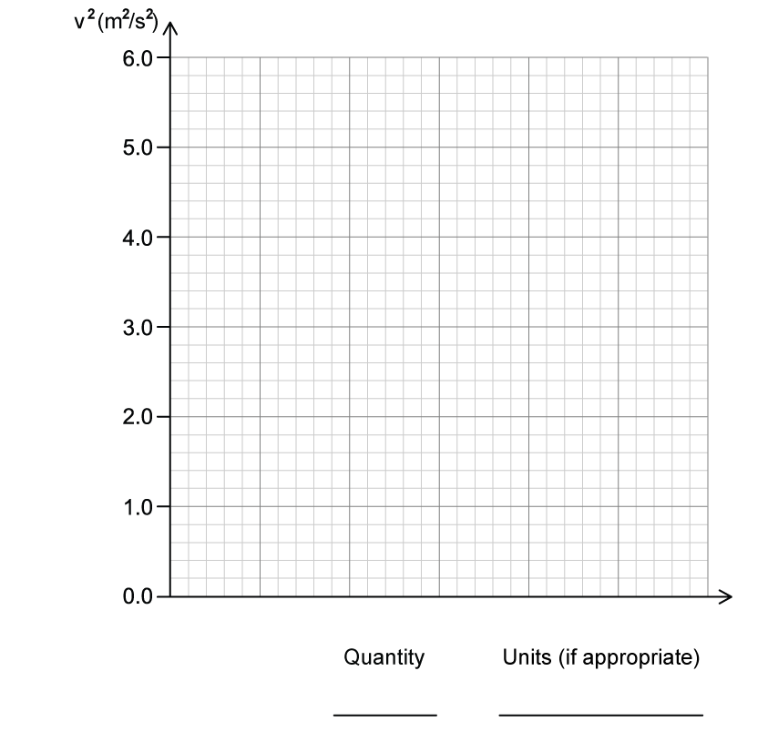
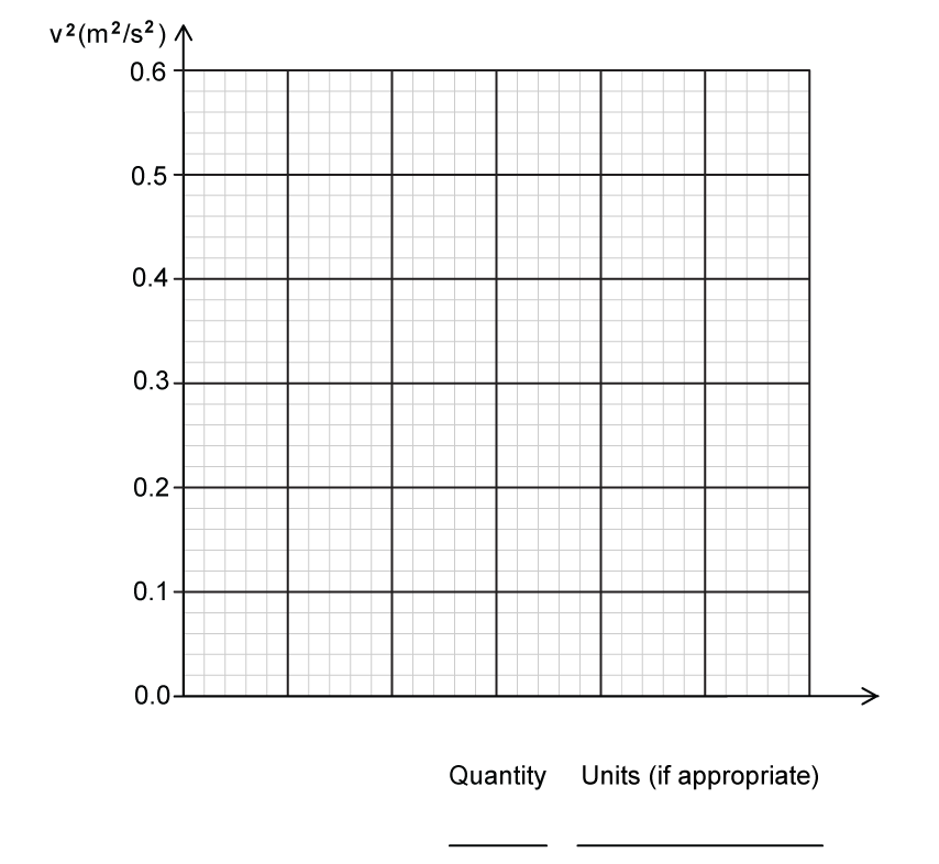
The students create a graph with plotted on the vertical axis.
i) Label the horizontal axis of Figure 3 with a measured or calculated quantity. Include units, as appropriate. The graphed quantities should yield a linear graph that can be used to determine an experimental value for the mass of the sphere.
ii) On the grid in Figure 3, create a graph of the quantities indicated in part c)i).
Clearly label the horizontal axis with a numerical scale
Plot the corresponding data points on the grid
Any columns added to Table 1 for scratch work will not be scored
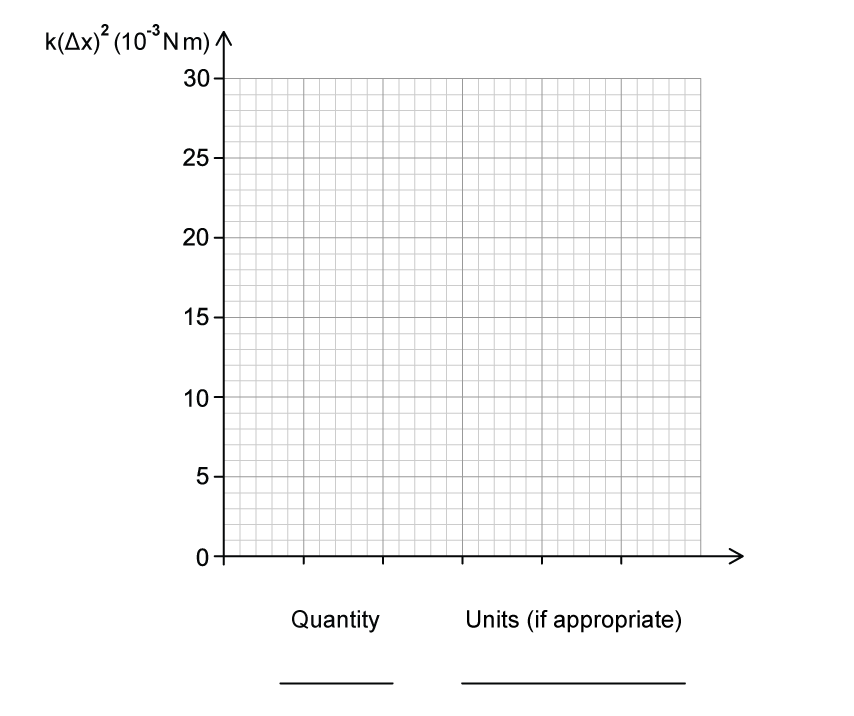
Figure 3
iii) Draw a best-fit line to the data graphed in part c)ii).
Calculate an experimental value for the mass of the sphere using the best-fit line that you drew in part c)iii).
Was this exam question helpful?