Price Elasticity of Supply (PES) (Cambridge (CIE) A Level Economics): Revision Note

Defining and calculating PES

• The law of supply states that when there is an increase in price (ceteris paribus), producers will increase the quantity supplied and vice versa

  • Economists are interested by how much the quantity supplied will increase

• Price elasticity of supply (PES) reveals how responsive the change in quantity supplied is to a change in price

  • The responsiveness is different for different types of products

Calculation of PES

• PES can be calculated using the following formula:

• To calculate a % change, use the following formula

Interpreting the PES coefficient

• The values of PES vary from 0 to infinity (∞) and they are classified as follows:

Value	Explanation
0 Perfectly price inelastic	The QS is completely unresponsive to a change in P (e.g. fixed number of seats in a theatre) so the supply curve is vertical
0→1 Relatively price inelastic	The %∆ in QS is less than proportional to the %∆ in P (e.g., agricultural products)
1→ ∞ Relatively price elastic	The %∆ in QS is more than proportional to the %∆ in P (e.g., t-shirts)
∞ Perfectly price elastic	The %∆ in QS will fall to zero with any %∆ in P However, supply is unlimited at a particular price This is a very theoretical scenario but is evident when examining international trade diagrams where the supply curve is horizontal
1 Unitary elasticity of supply	The value of PES: 1 The percentage change in quantity supplied is exactly equal to the percentage change in price Any supply curve that starts at the origin has unitary elasticity S1, S2 and S3 all have a PES value equal to 1 The %∆ in P = %∆ in QS

Factors that influence the PES

• Some products are more responsive to changes in price than others

• This responsiveness is known as Price Elasticity of Supply (PES)

• The factors that affect how responsive supply is, are called the determinants of PES

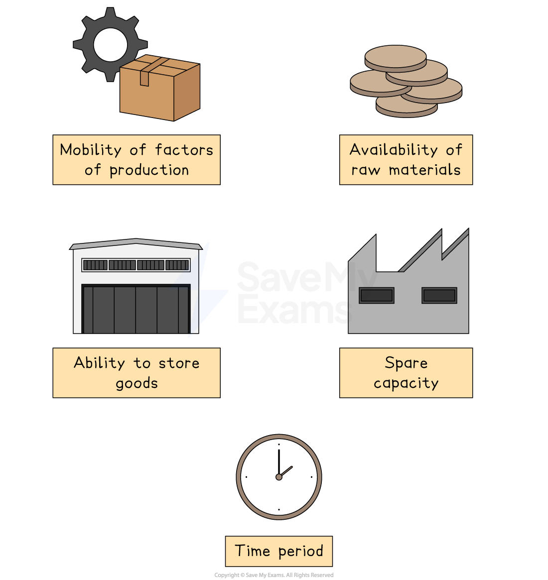
1. Mobility of the factors of production

• If producers can quickly switch resources (e.g., labour, capital) between products, then PES will be higher (elastic)

• If resources are specialised or fixed, then supply is less responsive (inelastic)

  • For example, if the price of hiking boots rises, a shoe manufacturer who can easily shift workers and machinery from making trainers to boots will have elastic supply

2. Availability of raw materials

• If raw materials are easily available, producers can respond quickly to price changes → elastic supply

• If materials are scarce or hard to obtain, supply cannot increase easily → inelastic supply

  • For example, a chocolate producer with limited access to cocoa beans may find it harder to increase supply when prices rise.

3. Ability to store stock

• If goods can be stored easily, producers can build up inventory and release more when prices rise → elastic supply

• If goods cannot be stored (e.g., fresh flowers), supply will be more inelastic

  • For example, producers of tinned food can respond quickly to price increases because the products can be stored for long periods

4. Spare capacity

• If a firm has unused capacity (idle machines, underused staff), it can increase output quickly when prices rise → elastic supply

• If operating at full capacity, it cannot easily raise production → inelastic supply

• For example, a car factory with extra machinery and space can respond rapidly to rising demand

5. Time period

• In the short run, supply is usually more inelastic because firms need time to adjust production

• In the long run, supply becomes more elastic as firms can invest in more resources and change production processes

• For example, avocado farmers cannot instantly grow more avocados when prices rise — but over time, they can plant more trees and expand supply

How PES affects business reactions to market changes

• Price Elasticity of Supply (PES) helps explain how quickly and easily businesses can adjust their output when market conditions shift

• A product with elastic supply can be increased quickly when prices rise, while inelastic supply means production is slower or harder to change

Manufactured goods: More flexible supply

• In the short term, businesses that produce manufactured items like trainers, headphones, or stationery, often have more flexibility

• If demand suddenly increases, they can release stock from warehouses or ramp up production with existing machinery.

  • For example, if a surge in demand for reusable water bottles occurs due to a sustainability trend, manufacturers can respond quickly by increasing output

• Over time, if the demand remains high, firms may invest in more equipment or hire additional staff to expand capacity

Agricultural products: Slower to respond

• Farming and food production tend to be less responsive in the short run

• Crops like strawberries or wheat cannot be grown overnight, and supply is affected by unpredictable factors such as weather, pests, or seasonal cycles

  • If demand for avocados spikes due to a health craze, farmers cannot instantly grow more. They must wait for the next harvest

• External influences also play a role. Disease outbreaks in livestock, droughts, or trade restrictions can disrupt supply. These factors make agricultural PES more inelastic compared to manufactured goods

Global impact of PES differences

• When supply is inelastic, even small changes in demand can cause big price swings

  • If global demand for cocoa rises and supply cannot keep up, prices may soar, affecting chocolate producers and consumers worldwide

  • In contrast, if demand for mobile phone cases increases, prices may stay stable because supply can adjust more easily

Comparing the PES of agricultural products and manufactured products

1. Mobility of the factors of production

2. The rate at which costs of production (marginal costs) increase

 3. The ability to store goods

4. Spare production capacity

5. Time period