Phase Portraits (DP IB Applications & Interpretation (AI)): Revision Note

Did this video help you?
Phase portraits
What is a phase portrait for a system of coupled differential equations?
Consider the system of coupled equations that can be represented in the matrix form
format('truetype')%3Bfont-weight%3Anormal%3Bfont-style%3Anormal%3B%7D%3C%2Fstyle%3E%3C%2Fdefs%3E%3Ctext%20font-family%3D%22math1dd165a6c6b5bc8158c57065d13%22%20font-size%3D%2212%22%20font-weight%3D%22bold%22%20text-anchor%3D%22middle%22%20x%3D%225.5%22%20y%3D%226%22%3E.%3C%2Ftext%3E%3Ctext%20font-family%3D%22Times%20New%20Roman%22%20font-size%3D%2218%22%20font-style%3D%22italic%22%20font-weight%3D%22bold%22%20text-anchor%3D%22middle%22%20x%3D%225.5%22%20y%3D%2218%22%3Ex%3C%2Ftext%3E%3Ctext%20font-family%3D%22math1dd165a6c6b5bc8158c57065d13%22%20font-size%3D%2216%22%20text-anchor%3D%22middle%22%20x%3D%2219.5%22%20y%3D%2218%22%3E%3D%3C%2Ftext%3E%3Ctext%20font-family%3D%22Times%20New%20Roman%22%20font-size%3D%2218%22%20font-style%3D%22italic%22%20font-weight%3D%22bold%22%20text-anchor%3D%22middle%22%20x%3D%2236.5%22%20y%3D%2218%22%3EM%3C%2Ftext%3E%3Ctext%20font-family%3D%22Times%20New%20Roman%22%20font-size%3D%2218%22%20font-style%3D%22italic%22%20font-weight%3D%22bold%22%20text-anchor%3D%22middle%22%20x%3D%2250.5%22%20y%3D%2218%22%3Ex%3C%2Ftext%3E%3C%2Fsvg%3E) , where
, where A phase portrait is a diagram showing how the values of x and y change over time
On a phase portrait we will usually sketch several typical solution trajectories
The precise trajectory that the solution for a particular system will travel along is determined by the initial conditions for the system
Suppose for the matrix

 and
and  are the eigenvalues
 and
and  are the corresponding eigenvectors
The overall nature of the phase portrait depends in large part on the values of
and
format('truetype')%3Bfont-weight%3Anormal%3Bfont-style%3Anormal%3B%7D%40font-face%7Bfont-family%3A'brack_sm2882ad605b1e27be87c7468'%3Bsrc%3Aurl(data%3Afont%2Ftruetype%3Bcharset%3Dutf-8%3Bbase64%2CAAEAAAAMAIAAAwBAT1MvMi7PH4UAAADMAAAATmNtYXA3kjw6AAABHAAAADxjdnQgAQYDiAAAAVgAAAASZ2x5ZkyYQ7YAAAFsAAAAkWhlYWQLyR8fAAACAAAAADZoaGVhAq0XCAAAAjgAAAAkaG10eDEjA%2FUAAAJcAAAADGxvY2EAAEKZAAACaAAAABBtYXhwBJsEcQAAAngAAAAgbmFtZW7QvZAAAAKYAAAB5XBvc3QArQBVAAAEgAAAACBwcmVwu5WEAAAABKAAAAAHAAACDAGQAAUAAAQABAAAAAAABAAEAAAAAAAAAQEAAAAAAAAAAAAAAAAAAAAAAAAAAAAAAAAAAAAAACAgICAAAAAg9AMD%2FP%2F8AAABVAABAAAAAAACAAEAAQAAABQAAwABAAAAFAAEACgAAAAGAAQAAQACI5wjn%2F%2F%2FAAAjnCOf%2F%2F%2FcZdxjAAEAAAAAAAAAAAFUAFQBAAArAIwAgACoAAcAAAACAAAAAADVAQEAAwAHAAAxMxEjFyM1M9XVq4CAAQHWqwABAAAAAABVAVgAAwAfGAGwAy%2BwADyxAgL1sAE8ALEDAD%2BwAjx8sQAG9bABPBEzESNVVQFY%2FqgAAQDXAAABLAFUAAMAIBgBsAUvsAE8sAI8sQAC9bADPACwAy%2BwAjyxAAH1sAE8EzMRI9dVVQFU%2FqwAAAAAAQAAAAEAAIsesexfDzz1AAMEAP%2F%2F%2F%2F%2FVre5k%2F%2F%2F%2F%2F9Wt7mT%2FgP%2F%2FAdYBWAAAAAoAAgABAAAAAAABAAABVP%2F%2FAAAXcP%2BA%2F4AB1gABAAAAAAAAAAAAAAAAAAAAAwDVAAABLAAAASwA1wAAAAAAAAAhAAAAWAAAAJEAAQAAAAMACgACAAAAAAACAIAEAAAAAAAEAABlAAAAAAAAABUBAgAAAAAAAAABACYAAAAAAAAAAAACAA4AJgAAAAAAAAADAEQANAAAAAAAAAAEACYAeAAAAAAAAAAFABYAngAAAAAAAAAGABMAtAAAAAAAAAAIABwAxwABAAAAAAABACYAAAABAAAAAAACAA4AJgABAAAAAAADAEQANAABAAAAAAAEACYAeAABAAAAAAAFABYAngABAAAAAAAGABMAtAABAAAAAAAIABwAxwADAAEECQABACYAAAADAAEECQACAA4AJgADAAEECQADAEQANAADAAEECQAEACYAeAADAAEECQAFABYAngADAAEECQAGABMAtAADAAEECQAIABwAxwBCAHIAYQBjAGsAZQB0AHMAIABzAG0AYQBsAGwAIABzAGkAegBlAFIAZQBnAHUAbABhAHIATQBhAHQAaABzACAARgBvAHIAIABNAG8AcgBlACAAQgByAGEAYwBrAGUAdABzACAAcwBtAGEAbABsACAAcwBpAHoAZQBCAHIAYQBjAGsAZQB0AHMAIABzAG0AYQBsAGwAIABzAGkAegBlAFYAZQByAHMAaQBvAG4AIAAyAC4AMEJyYWNrZXRzX3NtYWxsX3NpemUATQBhAHQAaABzACAARgBvAHIAIABNAG8AcgBlAAAAAAMAAAAAAAAAqgBVAAAAAAAAAAAAAAAAAAAAAAAAAAC5B%2F8AAo2FAA%3D%3D)format('truetype')%3Bfont-weight%3Anormal%3Bfont-style%3Anormal%3B%7D%40font-face%7Bfont-family%3A'bracketse552f5417ff4680c6b50499'%3Bsrc%3Aurl(data%3Afont%2Ftruetype%3Bcharset%3Dutf-8%3Bbase64%2CAAEAAAAMAIAAAwBAT1MvMi7RIisAAADMAAAATmNtYXBi7uzYAAABHAAAAExjdnQgBAkDLgAAAWgAAAASZ2x5Zo64f%2BkAAAF8AAABSWhlYWQLniGcAAACyAAAADZoaGVhBK4XLAAAAwAAAAAkaG10eCWq%2F90AAAMkAAAAFGxvY2EAABknAAADOAAAABhtYXhwBJIESAAAA1AAAAAgbmFtZRAA8I4AAANwAAAB3nBvc3QBwwDgAAAFUAAAACBwcmVwupWEAAAABXAAAAAHAAACggGQAAUAAAQABAAAAAAABAAEAAAAAAAAAQEAAAAAAAAAAAAAAAAAAAAAAAAAAAAAAAAAAAAAACAgICAAAAAg9AMEAAAAAAADgAAAAAAAAAACAAEAAQAAABQAAwABAAAAFAAEADgAAAAKAAgAAgACI5sjnSOeI6D%2F%2FwAAI5sjnSOeI6D%2F%2F9xm3GXcZdxkAAEAAAAAAAAAAAAAAAABVABWAQAALACoA4AAMgAHAAAAAgAAACoA1QNVAAMABwAANTMRIxMjETPV1auAgCoDK%2F0AAtUAAQAAAAABgAOAAAUAJBgBsAAvsAPFsQEC%2FbADELEEBP0AsQAAP7ABPLEEBj%2BwAzwwMTEzEAEjAFUBKyv%2BqwH8AYT%2BqgABAAAAAAGAA4AABQAmGAGwAC6wA8WxBQL9sAMQsQIE%2FQB8sQAGPxiwBTyxAwb2sAI8MDEREgEzABMBAVQr%2FtMCA4D91v6qAYQB%2FAAB%2F6wAAAEsA4AABQAnGAGwAC%2BwBzywA8WxAQL9sAMQsQQE%2FQCxAAA%2FsAE8sQQGP7ADPDAxISMSATMAASxVAf7UKwFVAfwBhP6rAAH%2FrAAAASwDgAAFACkYAbABL7AHPLAExbEAAv2wBBCxAwT9AHyxAQY%2FsAA8GLEEAD%2BwAzwwMRMzEAEjANdV%2FqsrASsDgP3V%2FqsBhgAAAAABAAAAAQAAeuTcpl8PPPUAAwQA%2F%2F%2F%2F%2F9Wt7o7%2F%2F%2F%2F%2F1a3ujv%2BsAAABgAOAAAAACgACAAEAAAAAAAEAAAOAAAAAABdw%2F6z%2FrAGAAAEAAAAAAAAAAAAAAAAAAAAFANUAAAEsAAABLAAAASz%2FrAEs%2F6wAAAAAAAAAJAAAAGgAAACzAAAA%2FQAAAUkAAQAAAAUACAACAAAAAAACAIAEAAAAAAAEAAA%2BAAAAAAAAABUBAgAAAAAAAAABACQAAAAAAAAAAAACAA4AJAAAAAAAAAADAEIAMgAAAAAAAAAEACQAdAAAAAAAAAAFABYAmAAAAAAAAAAGABIArgAAAAAAAAAIABwAwAABAAAAAAABACQAAAABAAAAAAACAA4AJAABAAAAAAADAEIAMgABAAAAAAAEACQAdAABAAAAAAAFABYAmAABAAAAAAAGABIArgABAAAAAAAIABwAwAADAAEECQABACQAAAADAAEECQACAA4AJAADAAEECQADAEIAMgADAAEECQAEACQAdAADAAEECQAFABYAmAADAAEECQAGABIArgADAAEECQAIABwAwABCAHIAYQBjAGsAZQB0AHMAIABmAHUAbABsACAAcwBpAHoAZQBSAGUAZwB1AGwAYQByAE0AYQB0AGgAcwAgAEYAbwByACAATQBvAHIAZQAgAEIAcgBhAGMAawBlAHQAcwAgAGYAdQBsAGwAIABzAGkAegBlAEIAcgBhAGMAawBlAHQAcwAgAGYAdQBsAGwAIABzAGkAegBlAFYAZQByAHMAaQBvAG4AIAAyAC4AMEJyYWNrZXRzX2Z1bGxfc2l6ZQBNAGEAdABoAHMAIABGAG8AcgAgAE0AbwByAGUAAAADAAAAAAAAAcAA4AAAAAAAAAAAAAAAAAAAAAAAAAAAuQf%2FAAGNhQA%3D)format('truetype')%3Bfont-weight%3Anormal%3Bfont-style%3Anormal%3B%7D%3C%2Fstyle%3E%3C%2Fdefs%3E%3Ctext%20font-family%3D%22math1dd165a6c6b5bc8158c57065d13%22%20font-size%3D%2212%22%20font-weight%3D%22bold%22%20text-anchor%3D%22middle%22%20x%3D%225.5%22%20y%3D%2223%22%3E.%3C%2Ftext%3E%3Ctext%20font-family%3D%22Times%20New%20Roman%22%20font-size%3D%2218%22%20font-style%3D%22italic%22%20font-weight%3D%22bold%22%20text-anchor%3D%22middle%22%20x%3D%225.5%22%20y%3D%2235%22%3Ex%3C%2Ftext%3E%3Ctext%20font-family%3D%22math1dd165a6c6b5bc8158c57065d13%22%20font-size%3D%2216%22%20text-anchor%3D%22middle%22%20x%3D%2219.5%22%20y%3D%2235%22%3E%3D%3C%2Ftext%3E%3Ctext%20font-family%3D%22bracketse552f5417ff4680c6b50499%22%20font-size%3D%2218%22%20text-anchor%3D%22start%22%20x%3D%2229.5%22%20y%3D%2217%22%3E%26%23x239B%3B%3C%2Ftext%3E%3Ctext%20font-family%3D%22brack_sm2882ad605b1e27be87c7468%22%20font-size%3D%2218%22%20text-anchor%3D%22start%22%20x%3D%2229.5%22%20y%3D%2223%22%3E%26%23x239C%3B%3C%2Ftext%3E%3Ctext%20font-family%3D%22brack_sm2882ad605b1e27be87c7468%22%20font-size%3D%2218%22%20text-anchor%3D%22start%22%20x%3D%2229.5%22%20y%3D%2229%22%3E%26%23x239C%3B%3C%2Ftext%3E%3Ctext%20font-family%3D%22brack_sm2882ad605b1e27be87c7468%22%20font-size%3D%2218%22%20text-anchor%3D%22start%22%20x%3D%2229.5%22%20y%3D%2235%22%3E%26%23x239C%3B%3C%2Ftext%3E%3Ctext%20font-family%3D%22brack_sm2882ad605b1e27be87c7468%22%20font-size%3D%2218%22%20text-anchor%3D%22start%22%20x%3D%2229.5%22%20y%3D%2241%22%3E%26%23x239C%3B%3C%2Ftext%3E%3Ctext%20font-family%3D%22bracketse552f5417ff4680c6b50499%22%20font-size%3D%2218%22%20text-anchor%3D%22start%22%20x%3D%2229.5%22%20y%3D%2257%22%3E%26%23x239D%3B%3C%2Ftext%3E%3Ctext%20font-family%3D%22bracketse552f5417ff4680c6b50499%22%20font-size%3D%2218%22%20text-anchor%3D%22start%22%20x%3D%2254.5%22%20y%3D%2217%22%3E%26%23x239E%3B%3C%2Ftext%3E%3Ctext%20font-family%3D%22brack_sm2882ad605b1e27be87c7468%22%20font-size%3D%2218%22%20text-anchor%3D%22start%22%20x%3D%2254.5%22%20y%3D%2223%22%3E%26%23x239F%3B%3C%2Ftext%3E%3Ctext%20font-family%3D%22brack_sm2882ad605b1e27be87c7468%22%20font-size%3D%2218%22%20text-anchor%3D%22start%22%20x%3D%2254.5%22%20y%3D%2229%22%3E%26%23x239F%3B%3C%2Ftext%3E%3Ctext%20font-family%3D%22brack_sm2882ad605b1e27be87c7468%22%20font-size%3D%2218%22%20text-anchor%3D%22start%22%20x%3D%2254.5%22%20y%3D%2235%22%3E%26%23x239F%3B%3C%2Ftext%3E%3Ctext%20font-family%3D%22brack_sm2882ad605b1e27be87c7468%22%20font-size%3D%2218%22%20text-anchor%3D%22start%22%20x%3D%2254.5%22%20y%3D%2241%22%3E%26%23x239F%3B%3C%2Ftext%3E%3Ctext%20font-family%3D%22bracketse552f5417ff4680c6b50499%22%20font-size%3D%2218%22%20text-anchor%3D%22start%22%20x%3D%2254.5%22%20y%3D%2257%22%3E%26%23x23A0%3B%3C%2Ftext%3E%3Ctext%20font-family%3D%22math1dd165a6c6b5bc8158c57065d13%22%20font-size%3D%2212%22%20text-anchor%3D%22middle%22%20x%3D%2244.5%22%20y%3D%2210%22%3E.%3C%2Ftext%3E%3Ctext%20font-family%3D%22Times%20New%20Roman%22%20font-size%3D%2218%22%20font-style%3D%22italic%22%20text-anchor%3D%22middle%22%20x%3D%2243.5%22%20y%3D%2221%22%3Ex%3C%2Ftext%3E%3Ctext%20font-family%3D%22math1dd165a6c6b5bc8158c57065d13%22%20font-size%3D%2212%22%20text-anchor%3D%22middle%22%20x%3D%2244.5%22%20y%3D%2238%22%3E.%3C%2Ftext%3E%3Ctext%20font-family%3D%22Times%20New%20Roman%22%20font-size%3D%2218%22%20font-style%3D%22italic%22%20text-anchor%3D%22middle%22%20x%3D%2243.5%22%20y%3D%2249%22%3Ey%3C%2Ftext%3E%3C%2Fsvg%3E)
format('truetype')%3Bfont-weight%3Anormal%3Bfont-style%3Anormal%3B%7D%40font-face%7Bfont-family%3A'brack_sm2882ad605b1e27be87c7468'%3Bsrc%3Aurl(data%3Afont%2Ftruetype%3Bcharset%3Dutf-8%3Bbase64%2CAAEAAAAMAIAAAwBAT1MvMi7PH4UAAADMAAAATmNtYXA3kjw6AAABHAAAADxjdnQgAQYDiAAAAVgAAAASZ2x5ZkyYQ7YAAAFsAAAAkWhlYWQLyR8fAAACAAAAADZoaGVhAq0XCAAAAjgAAAAkaG10eDEjA%2FUAAAJcAAAADGxvY2EAAEKZAAACaAAAABBtYXhwBJsEcQAAAngAAAAgbmFtZW7QvZAAAAKYAAAB5XBvc3QArQBVAAAEgAAAACBwcmVwu5WEAAAABKAAAAAHAAACDAGQAAUAAAQABAAAAAAABAAEAAAAAAAAAQEAAAAAAAAAAAAAAAAAAAAAAAAAAAAAAAAAAAAAACAgICAAAAAg9AMD%2FP%2F8AAABVAABAAAAAAACAAEAAQAAABQAAwABAAAAFAAEACgAAAAGAAQAAQACI5wjn%2F%2F%2FAAAjnCOf%2F%2F%2FcZdxjAAEAAAAAAAAAAAFUAFQBAAArAIwAgACoAAcAAAACAAAAAADVAQEAAwAHAAAxMxEjFyM1M9XVq4CAAQHWqwABAAAAAABVAVgAAwAfGAGwAy%2BwADyxAgL1sAE8ALEDAD%2BwAjx8sQAG9bABPBEzESNVVQFY%2FqgAAQDXAAABLAFUAAMAIBgBsAUvsAE8sAI8sQAC9bADPACwAy%2BwAjyxAAH1sAE8EzMRI9dVVQFU%2FqwAAAAAAQAAAAEAAIsesexfDzz1AAMEAP%2F%2F%2F%2F%2FVre5k%2F%2F%2F%2F%2F9Wt7mT%2FgP%2F%2FAdYBWAAAAAoAAgABAAAAAAABAAABVP%2F%2FAAAXcP%2BA%2F4AB1gABAAAAAAAAAAAAAAAAAAAAAwDVAAABLAAAASwA1wAAAAAAAAAhAAAAWAAAAJEAAQAAAAMACgACAAAAAAACAIAEAAAAAAAEAABlAAAAAAAAABUBAgAAAAAAAAABACYAAAAAAAAAAAACAA4AJgAAAAAAAAADAEQANAAAAAAAAAAEACYAeAAAAAAAAAAFABYAngAAAAAAAAAGABMAtAAAAAAAAAAIABwAxwABAAAAAAABACYAAAABAAAAAAACAA4AJgABAAAAAAADAEQANAABAAAAAAAEACYAeAABAAAAAAAFABYAngABAAAAAAAGABMAtAABAAAAAAAIABwAxwADAAEECQABACYAAAADAAEECQACAA4AJgADAAEECQADAEQANAADAAEECQAEACYAeAADAAEECQAFABYAngADAAEECQAGABMAtAADAAEECQAIABwAxwBCAHIAYQBjAGsAZQB0AHMAIABzAG0AYQBsAGwAIABzAGkAegBlAFIAZQBnAHUAbABhAHIATQBhAHQAaABzACAARgBvAHIAIABNAG8AcgBlACAAQgByAGEAYwBrAGUAdABzACAAcwBtAGEAbABsACAAcwBpAHoAZQBCAHIAYQBjAGsAZQB0AHMAIABzAG0AYQBsAGwAIABzAGkAegBlAFYAZQByAHMAaQBvAG4AIAAyAC4AMEJyYWNrZXRzX3NtYWxsX3NpemUATQBhAHQAaABzACAARgBvAHIAIABNAG8AcgBlAAAAAAMAAAAAAAAAqgBVAAAAAAAAAAAAAAAAAAAAAAAAAAC5B%2F8AAo2FAA%3D%3D)format('truetype')%3Bfont-weight%3Anormal%3Bfont-style%3Anormal%3B%7D%40font-face%7Bfont-family%3A'bracketse552f5417ff4680c6b50499'%3Bsrc%3Aurl(data%3Afont%2Ftruetype%3Bcharset%3Dutf-8%3Bbase64%2CAAEAAAAMAIAAAwBAT1MvMi7RIisAAADMAAAATmNtYXBi7uzYAAABHAAAAExjdnQgBAkDLgAAAWgAAAASZ2x5Zo64f%2BkAAAF8AAABSWhlYWQLniGcAAACyAAAADZoaGVhBK4XLAAAAwAAAAAkaG10eCWq%2F90AAAMkAAAAFGxvY2EAABknAAADOAAAABhtYXhwBJIESAAAA1AAAAAgbmFtZRAA8I4AAANwAAAB3nBvc3QBwwDgAAAFUAAAACBwcmVwupWEAAAABXAAAAAHAAACggGQAAUAAAQABAAAAAAABAAEAAAAAAAAAQEAAAAAAAAAAAAAAAAAAAAAAAAAAAAAAAAAAAAAACAgICAAAAAg9AMEAAAAAAADgAAAAAAAAAACAAEAAQAAABQAAwABAAAAFAAEADgAAAAKAAgAAgACI5sjnSOeI6D%2F%2FwAAI5sjnSOeI6D%2F%2F9xm3GXcZdxkAAEAAAAAAAAAAAAAAAABVABWAQAALACoA4AAMgAHAAAAAgAAACoA1QNVAAMABwAANTMRIxMjETPV1auAgCoDK%2F0AAtUAAQAAAAABgAOAAAUAJBgBsAAvsAPFsQEC%2FbADELEEBP0AsQAAP7ABPLEEBj%2BwAzwwMTEzEAEjAFUBKyv%2BqwH8AYT%2BqgABAAAAAAGAA4AABQAmGAGwAC6wA8WxBQL9sAMQsQIE%2FQB8sQAGPxiwBTyxAwb2sAI8MDEREgEzABMBAVQr%2FtMCA4D91v6qAYQB%2FAAB%2F6wAAAEsA4AABQAnGAGwAC%2BwBzywA8WxAQL9sAMQsQQE%2FQCxAAA%2FsAE8sQQGP7ADPDAxISMSATMAASxVAf7UKwFVAfwBhP6rAAH%2FrAAAASwDgAAFACkYAbABL7AHPLAExbEAAv2wBBCxAwT9AHyxAQY%2FsAA8GLEEAD%2BwAzwwMRMzEAEjANdV%2FqsrASsDgP3V%2FqsBhgAAAAABAAAAAQAAeuTcpl8PPPUAAwQA%2F%2F%2F%2F%2F9Wt7o7%2F%2F%2F%2F%2F1a3ujv%2BsAAABgAOAAAAACgACAAEAAAAAAAEAAAOAAAAAABdw%2F6z%2FrAGAAAEAAAAAAAAAAAAAAAAAAAAFANUAAAEsAAABLAAAASz%2FrAEs%2F6wAAAAAAAAAJAAAAGgAAACzAAAA%2FQAAAUkAAQAAAAUACAACAAAAAAACAIAEAAAAAAAEAAA%2BAAAAAAAAABUBAgAAAAAAAAABACQAAAAAAAAAAAACAA4AJAAAAAAAAAADAEIAMgAAAAAAAAAEACQAdAAAAAAAAAAFABYAmAAAAAAAAAAGABIArgAAAAAAAAAIABwAwAABAAAAAAABACQAAAABAAAAAAACAA4AJAABAAAAAAADAEIAMgABAAAAAAAEACQAdAABAAAAAAAFABYAmAABAAAAAAAGABIArgABAAAAAAAIABwAwAADAAEECQABACQAAAADAAEECQACAA4AJAADAAEECQADAEIAMgADAAEECQAEACQAdAADAAEECQAFABYAmAADAAEECQAGABIArgADAAEECQAIABwAwABCAHIAYQBjAGsAZQB0AHMAIABmAHUAbABsACAAcwBpAHoAZQBSAGUAZwB1AGwAYQByAE0AYQB0AGgAcwAgAEYAbwByACAATQBvAHIAZQAgAEIAcgBhAGMAawBlAHQAcwAgAGYAdQBsAGwAIABzAGkAegBlAEIAcgBhAGMAawBlAHQAcwAgAGYAdQBsAGwAIABzAGkAegBlAFYAZQByAHMAaQBvAG4AIAAyAC4AMEJyYWNrZXRzX2Z1bGxfc2l6ZQBNAGEAdABoAHMAIABGAG8AcgAgAE0AbwByAGUAAAADAAAAAAAAAcAA4AAAAAAAAAAAAAAAAAAAAAAAAAAAuQf%2FAAGNhQA%3D)format('truetype')%3Bfont-weight%3Anormal%3Bfont-style%3Anormal%3B%7D%3C%2Fstyle%3E%3C%2Fdefs%3E%3Ctext%20font-family%3D%22Times%20New%20Roman%22%20font-size%3D%2218%22%20font-style%3D%22italic%22%20font-weight%3D%22bold%22%20text-anchor%3D%22middle%22%20x%3D%228.5%22%20y%3D%2233%22%3EM%3C%2Ftext%3E%3Ctext%20font-family%3D%22math17f39f8317fbdb1988ef4c628eb%22%20font-size%3D%2216%22%20text-anchor%3D%22middle%22%20x%3D%2226.5%22%20y%3D%2233%22%3E%3D%3C%2Ftext%3E%3Ctext%20font-family%3D%22bracketse552f5417ff4680c6b50499%22%20font-size%3D%2218%22%20text-anchor%3D%22start%22%20x%3D%2236.5%22%20y%3D%2218%22%3E%26%23x239B%3B%3C%2Ftext%3E%3Ctext%20font-family%3D%22brack_sm2882ad605b1e27be87c7468%22%20font-size%3D%2218%22%20text-anchor%3D%22start%22%20x%3D%2236.5%22%20y%3D%2224%22%3E%26%23x239C%3B%3C%2Ftext%3E%3Ctext%20font-family%3D%22brack_sm2882ad605b1e27be87c7468%22%20font-size%3D%2218%22%20text-anchor%3D%22start%22%20x%3D%2236.5%22%20y%3D%2230%22%3E%26%23x239C%3B%3C%2Ftext%3E%3Ctext%20font-family%3D%22brack_sm2882ad605b1e27be87c7468%22%20font-size%3D%2218%22%20text-anchor%3D%22start%22%20x%3D%2236.5%22%20y%3D%2236%22%3E%26%23x239C%3B%3C%2Ftext%3E%3Ctext%20font-family%3D%22bracketse552f5417ff4680c6b50499%22%20font-size%3D%2218%22%20text-anchor%3D%22start%22%20x%3D%2236.5%22%20y%3D%2252%22%3E%26%23x239D%3B%3C%2Ftext%3E%3Ctext%20font-family%3D%22bracketse552f5417ff4680c6b50499%22%20font-size%3D%2218%22%20text-anchor%3D%22start%22%20x%3D%2278.5%22%20y%3D%2218%22%3E%26%23x239E%3B%3C%2Ftext%3E%3Ctext%20font-family%3D%22brack_sm2882ad605b1e27be87c7468%22%20font-size%3D%2218%22%20text-anchor%3D%22start%22%20x%3D%2278.5%22%20y%3D%2224%22%3E%26%23x239F%3B%3C%2Ftext%3E%3Ctext%20font-family%3D%22brack_sm2882ad605b1e27be87c7468%22%20font-size%3D%2218%22%20text-anchor%3D%22start%22%20x%3D%2278.5%22%20y%3D%2230%22%3E%26%23x239F%3B%3C%2Ftext%3E%3Ctext%20font-family%3D%22brack_sm2882ad605b1e27be87c7468%22%20font-size%3D%2218%22%20text-anchor%3D%22start%22%20x%3D%2278.5%22%20y%3D%2236%22%3E%26%23x239F%3B%3C%2Ftext%3E%3Ctext%20font-family%3D%22bracketse552f5417ff4680c6b50499%22%20font-size%3D%2218%22%20text-anchor%3D%22start%22%20x%3D%2278.5%22%20y%3D%2252%22%3E%26%23x23A0%3B%3C%2Ftext%3E%3Ctext%20font-family%3D%22Times%20New%20Roman%22%20font-size%3D%2218%22%20font-style%3D%22italic%22%20text-anchor%3D%22middle%22%20x%3D%2250.5%22%20y%3D%2219%22%3Ea%3C%2Ftext%3E%3Ctext%20font-family%3D%22Times%20New%20Roman%22%20font-size%3D%2218%22%20font-style%3D%22italic%22%20text-anchor%3D%22middle%22%20x%3D%2267.5%22%20y%3D%2219%22%3Eb%3C%2Ftext%3E%3Ctext%20font-family%3D%22Times%20New%20Roman%22%20font-size%3D%2218%22%20font-style%3D%22italic%22%20text-anchor%3D%22middle%22%20x%3D%2250.5%22%20y%3D%2245%22%3Ec%3C%2Ftext%3E%3Ctext%20font-family%3D%22Times%20New%20Roman%22%20font-size%3D%2218%22%20font-style%3D%22italic%22%20text-anchor%3D%22middle%22%20x%3D%2267.5%22%20y%3D%2245%22%3Ed%3C%2Ftext%3E%3C%2Fsvg%3E)
format('truetype')%3Bfont-weight%3Anormal%3Bfont-style%3Anormal%3B%7D%40font-face%7Bfont-family%3A'brack_sm2882ad605b1e27be87c7468'%3Bsrc%3Aurl(data%3Afont%2Ftruetype%3Bcharset%3Dutf-8%3Bbase64%2CAAEAAAAMAIAAAwBAT1MvMi7PH4UAAADMAAAATmNtYXA3kjw6AAABHAAAADxjdnQgAQYDiAAAAVgAAAASZ2x5ZkyYQ7YAAAFsAAAAkWhlYWQLyR8fAAACAAAAADZoaGVhAq0XCAAAAjgAAAAkaG10eDEjA%2FUAAAJcAAAADGxvY2EAAEKZAAACaAAAABBtYXhwBJsEcQAAAngAAAAgbmFtZW7QvZAAAAKYAAAB5XBvc3QArQBVAAAEgAAAACBwcmVwu5WEAAAABKAAAAAHAAACDAGQAAUAAAQABAAAAAAABAAEAAAAAAAAAQEAAAAAAAAAAAAAAAAAAAAAAAAAAAAAAAAAAAAAACAgICAAAAAg9AMD%2FP%2F8AAABVAABAAAAAAACAAEAAQAAABQAAwABAAAAFAAEACgAAAAGAAQAAQACI5wjn%2F%2F%2FAAAjnCOf%2F%2F%2FcZdxjAAEAAAAAAAAAAAFUAFQBAAArAIwAgACoAAcAAAACAAAAAADVAQEAAwAHAAAxMxEjFyM1M9XVq4CAAQHWqwABAAAAAABVAVgAAwAfGAGwAy%2BwADyxAgL1sAE8ALEDAD%2BwAjx8sQAG9bABPBEzESNVVQFY%2FqgAAQDXAAABLAFUAAMAIBgBsAUvsAE8sAI8sQAC9bADPACwAy%2BwAjyxAAH1sAE8EzMRI9dVVQFU%2FqwAAAAAAQAAAAEAAIsesexfDzz1AAMEAP%2F%2F%2F%2F%2FVre5k%2F%2F%2F%2F%2F9Wt7mT%2FgP%2F%2FAdYBWAAAAAoAAgABAAAAAAABAAABVP%2F%2FAAAXcP%2BA%2F4AB1gABAAAAAAAAAAAAAAAAAAAAAwDVAAABLAAAASwA1wAAAAAAAAAhAAAAWAAAAJEAAQAAAAMACgACAAAAAAACAIAEAAAAAAAEAABlAAAAAAAAABUBAgAAAAAAAAABACYAAAAAAAAAAAACAA4AJgAAAAAAAAADAEQANAAAAAAAAAAEACYAeAAAAAAAAAAFABYAngAAAAAAAAAGABMAtAAAAAAAAAAIABwAxwABAAAAAAABACYAAAABAAAAAAACAA4AJgABAAAAAAADAEQANAABAAAAAAAEACYAeAABAAAAAAAFABYAngABAAAAAAAGABMAtAABAAAAAAAIABwAxwADAAEECQABACYAAAADAAEECQACAA4AJgADAAEECQADAEQANAADAAEECQAEACYAeAADAAEECQAFABYAngADAAEECQAGABMAtAADAAEECQAIABwAxwBCAHIAYQBjAGsAZQB0AHMAIABzAG0AYQBsAGwAIABzAGkAegBlAFIAZQBnAHUAbABhAHIATQBhAHQAaABzACAARgBvAHIAIABNAG8AcgBlACAAQgByAGEAYwBrAGUAdABzACAAcwBtAGEAbABsACAAcwBpAHoAZQBCAHIAYQBjAGsAZQB0AHMAIABzAG0AYQBsAGwAIABzAGkAegBlAFYAZQByAHMAaQBvAG4AIAAyAC4AMEJyYWNrZXRzX3NtYWxsX3NpemUATQBhAHQAaABzACAARgBvAHIAIABNAG8AcgBlAAAAAAMAAAAAAAAAqgBVAAAAAAAAAAAAAAAAAAAAAAAAAAC5B%2F8AAo2FAA%3D%3D)format('truetype')%3Bfont-weight%3Anormal%3Bfont-style%3Anormal%3B%7D%40font-face%7Bfont-family%3A'bracketse552f5417ff4680c6b50499'%3Bsrc%3Aurl(data%3Afont%2Ftruetype%3Bcharset%3Dutf-8%3Bbase64%2CAAEAAAAMAIAAAwBAT1MvMi7RIisAAADMAAAATmNtYXBi7uzYAAABHAAAAExjdnQgBAkDLgAAAWgAAAASZ2x5Zo64f%2BkAAAF8AAABSWhlYWQLniGcAAACyAAAADZoaGVhBK4XLAAAAwAAAAAkaG10eCWq%2F90AAAMkAAAAFGxvY2EAABknAAADOAAAABhtYXhwBJIESAAAA1AAAAAgbmFtZRAA8I4AAANwAAAB3nBvc3QBwwDgAAAFUAAAACBwcmVwupWEAAAABXAAAAAHAAACggGQAAUAAAQABAAAAAAABAAEAAAAAAAAAQEAAAAAAAAAAAAAAAAAAAAAAAAAAAAAAAAAAAAAACAgICAAAAAg9AMEAAAAAAADgAAAAAAAAAACAAEAAQAAABQAAwABAAAAFAAEADgAAAAKAAgAAgACI5sjnSOeI6D%2F%2FwAAI5sjnSOeI6D%2F%2F9xm3GXcZdxkAAEAAAAAAAAAAAAAAAABVABWAQAALACoA4AAMgAHAAAAAgAAACoA1QNVAAMABwAANTMRIxMjETPV1auAgCoDK%2F0AAtUAAQAAAAABgAOAAAUAJBgBsAAvsAPFsQEC%2FbADELEEBP0AsQAAP7ABPLEEBj%2BwAzwwMTEzEAEjAFUBKyv%2BqwH8AYT%2BqgABAAAAAAGAA4AABQAmGAGwAC6wA8WxBQL9sAMQsQIE%2FQB8sQAGPxiwBTyxAwb2sAI8MDEREgEzABMBAVQr%2FtMCA4D91v6qAYQB%2FAAB%2F6wAAAEsA4AABQAnGAGwAC%2BwBzywA8WxAQL9sAMQsQQE%2FQCxAAA%2FsAE8sQQGP7ADPDAxISMSATMAASxVAf7UKwFVAfwBhP6rAAH%2FrAAAASwDgAAFACkYAbABL7AHPLAExbEAAv2wBBCxAwT9AHyxAQY%2FsAA8GLEEAD%2BwAzwwMRMzEAEjANdV%2FqsrASsDgP3V%2FqsBhgAAAAABAAAAAQAAeuTcpl8PPPUAAwQA%2F%2F%2F%2F%2F9Wt7o7%2F%2F%2F%2F%2F1a3ujv%2BsAAABgAOAAAAACgACAAEAAAAAAAEAAAOAAAAAABdw%2F6z%2FrAGAAAEAAAAAAAAAAAAAAAAAAAAFANUAAAEsAAABLAAAASz%2FrAEs%2F6wAAAAAAAAAJAAAAGgAAACzAAAA%2FQAAAUkAAQAAAAUACAACAAAAAAACAIAEAAAAAAAEAAA%2BAAAAAAAAABUBAgAAAAAAAAABACQAAAAAAAAAAAACAA4AJAAAAAAAAAADAEIAMgAAAAAAAAAEACQAdAAAAAAAAAAFABYAmAAAAAAAAAAGABIArgAAAAAAAAAIABwAwAABAAAAAAABACQAAAABAAAAAAACAA4AJAABAAAAAAADAEIAMgABAAAAAAAEACQAdAABAAAAAAAFABYAmAABAAAAAAAGABIArgABAAAAAAAIABwAwAADAAEECQABACQAAAADAAEECQACAA4AJAADAAEECQADAEIAMgADAAEECQAEACQAdAADAAEECQAFABYAmAADAAEECQAGABIArgADAAEECQAIABwAwABCAHIAYQBjAGsAZQB0AHMAIABmAHUAbABsACAAcwBpAHoAZQBSAGUAZwB1AGwAYQByAE0AYQB0AGgAcwAgAEYAbwByACAATQBvAHIAZQAgAEIAcgBhAGMAawBlAHQAcwAgAGYAdQBsAGwAIABzAGkAegBlAEIAcgBhAGMAawBlAHQAcwAgAGYAdQBsAGwAIABzAGkAegBlAFYAZQByAHMAaQBvAG4AIAAyAC4AMEJyYWNrZXRzX2Z1bGxfc2l6ZQBNAGEAdABoAHMAIABGAG8AcgAgAE0AbwByAGUAAAADAAAAAAAAAcAA4AAAAAAAAAAAAAAAAAAAAAAAAAAAuQf%2FAAGNhQA%3D)format('truetype')%3Bfont-weight%3Anormal%3Bfont-style%3Anormal%3B%7D%3C%2Fstyle%3E%3C%2Fdefs%3E%3Ctext%20font-family%3D%22Times%20New%20Roman%22%20font-size%3D%2218%22%20font-style%3D%22italic%22%20font-weight%3D%22bold%22%20text-anchor%3D%22middle%22%20x%3D%225.5%22%20y%3D%2233%22%3Ex%3C%2Ftext%3E%3Ctext%20font-family%3D%22math17f39f8317fbdb1988ef4c628eb%22%20font-size%3D%2216%22%20text-anchor%3D%22middle%22%20x%3D%2219.5%22%20y%3D%2233%22%3E%3D%3C%2Ftext%3E%3Ctext%20font-family%3D%22bracketse552f5417ff4680c6b50499%22%20font-size%3D%2218%22%20text-anchor%3D%22start%22%20x%3D%2229.5%22%20y%3D%2218%22%3E%26%23x239B%3B%3C%2Ftext%3E%3Ctext%20font-family%3D%22brack_sm2882ad605b1e27be87c7468%22%20font-size%3D%2218%22%20text-anchor%3D%22start%22%20x%3D%2229.5%22%20y%3D%2224%22%3E%26%23x239C%3B%3C%2Ftext%3E%3Ctext%20font-family%3D%22brack_sm2882ad605b1e27be87c7468%22%20font-size%3D%2218%22%20text-anchor%3D%22start%22%20x%3D%2229.5%22%20y%3D%2230%22%3E%26%23x239C%3B%3C%2Ftext%3E%3Ctext%20font-family%3D%22brack_sm2882ad605b1e27be87c7468%22%20font-size%3D%2218%22%20text-anchor%3D%22start%22%20x%3D%2229.5%22%20y%3D%2236%22%3E%26%23x239C%3B%3C%2Ftext%3E%3Ctext%20font-family%3D%22bracketse552f5417ff4680c6b50499%22%20font-size%3D%2218%22%20text-anchor%3D%22start%22%20x%3D%2229.5%22%20y%3D%2252%22%3E%26%23x239D%3B%3C%2Ftext%3E%3Ctext%20font-family%3D%22bracketse552f5417ff4680c6b50499%22%20font-size%3D%2218%22%20text-anchor%3D%22start%22%20x%3D%2254.5%22%20y%3D%2218%22%3E%26%23x239E%3B%3C%2Ftext%3E%3Ctext%20font-family%3D%22brack_sm2882ad605b1e27be87c7468%22%20font-size%3D%2218%22%20text-anchor%3D%22start%22%20x%3D%2254.5%22%20y%3D%2224%22%3E%26%23x239F%3B%3C%2Ftext%3E%3Ctext%20font-family%3D%22brack_sm2882ad605b1e27be87c7468%22%20font-size%3D%2218%22%20text-anchor%3D%22start%22%20x%3D%2254.5%22%20y%3D%2230%22%3E%26%23x239F%3B%3C%2Ftext%3E%3Ctext%20font-family%3D%22brack_sm2882ad605b1e27be87c7468%22%20font-size%3D%2218%22%20text-anchor%3D%22start%22%20x%3D%2254.5%22%20y%3D%2236%22%3E%26%23x239F%3B%3C%2Ftext%3E%3Ctext%20font-family%3D%22bracketse552f5417ff4680c6b50499%22%20font-size%3D%2218%22%20text-anchor%3D%22start%22%20x%3D%2254.5%22%20y%3D%2252%22%3E%26%23x23A0%3B%3C%2Ftext%3E%3Ctext%20font-family%3D%22Times%20New%20Roman%22%20font-size%3D%2218%22%20font-style%3D%22italic%22%20text-anchor%3D%22middle%22%20x%3D%2243.5%22%20y%3D%2219%22%3Ex%3C%2Ftext%3E%3Ctext%20font-family%3D%22Times%20New%20Roman%22%20font-size%3D%2218%22%20font-style%3D%22italic%22%20text-anchor%3D%22middle%22%20x%3D%2243.5%22%20y%3D%2245%22%3Ey%3C%2Ftext%3E%3C%2Fsvg%3E)
Examiner Tips and Tricks
You need to know how phase portraits looks when the eigenvalues or:
real, distinct and non-zero
complex conjugates
What does the phase portrait look like when the eigenvalues are real numbers?
The phase portraits when the eigenvalues are real always include two lines representing the eigenvectors
These go through the origin
They are parallel to the eigenvectors
The origin separates these two lines into four solution trajectories
For example, if
format('truetype')%3Bfont-weight%3Anormal%3Bfont-style%3Anormal%3B%7D%40font-face%7Bfont-family%3A'brack_sm2882ad605b1e27be87c7468'%3Bsrc%3Aurl(data%3Afont%2Ftruetype%3Bcharset%3Dutf-8%3Bbase64%2CAAEAAAAMAIAAAwBAT1MvMi7PH4UAAADMAAAATmNtYXA3kjw6AAABHAAAADxjdnQgAQYDiAAAAVgAAAASZ2x5ZkyYQ7YAAAFsAAAAkWhlYWQLyR8fAAACAAAAADZoaGVhAq0XCAAAAjgAAAAkaG10eDEjA%2FUAAAJcAAAADGxvY2EAAEKZAAACaAAAABBtYXhwBJsEcQAAAngAAAAgbmFtZW7QvZAAAAKYAAAB5XBvc3QArQBVAAAEgAAAACBwcmVwu5WEAAAABKAAAAAHAAACDAGQAAUAAAQABAAAAAAABAAEAAAAAAAAAQEAAAAAAAAAAAAAAAAAAAAAAAAAAAAAAAAAAAAAACAgICAAAAAg9AMD%2FP%2F8AAABVAABAAAAAAACAAEAAQAAABQAAwABAAAAFAAEACgAAAAGAAQAAQACI5wjn%2F%2F%2FAAAjnCOf%2F%2F%2FcZdxjAAEAAAAAAAAAAAFUAFQBAAArAIwAgACoAAcAAAACAAAAAADVAQEAAwAHAAAxMxEjFyM1M9XVq4CAAQHWqwABAAAAAABVAVgAAwAfGAGwAy%2BwADyxAgL1sAE8ALEDAD%2BwAjx8sQAG9bABPBEzESNVVQFY%2FqgAAQDXAAABLAFUAAMAIBgBsAUvsAE8sAI8sQAC9bADPACwAy%2BwAjyxAAH1sAE8EzMRI9dVVQFU%2FqwAAAAAAQAAAAEAAIsesexfDzz1AAMEAP%2F%2F%2F%2F%2FVre5k%2F%2F%2F%2F%2F9Wt7mT%2FgP%2F%2FAdYBWAAAAAoAAgABAAAAAAABAAABVP%2F%2FAAAXcP%2BA%2F4AB1gABAAAAAAAAAAAAAAAAAAAAAwDVAAABLAAAASwA1wAAAAAAAAAhAAAAWAAAAJEAAQAAAAMACgACAAAAAAACAIAEAAAAAAAEAABlAAAAAAAAABUBAgAAAAAAAAABACYAAAAAAAAAAAACAA4AJgAAAAAAAAADAEQANAAAAAAAAAAEACYAeAAAAAAAAAAFABYAngAAAAAAAAAGABMAtAAAAAAAAAAIABwAxwABAAAAAAABACYAAAABAAAAAAACAA4AJgABAAAAAAADAEQANAABAAAAAAAEACYAeAABAAAAAAAFABYAngABAAAAAAAGABMAtAABAAAAAAAIABwAxwADAAEECQABACYAAAADAAEECQACAA4AJgADAAEECQADAEQANAADAAEECQAEACYAeAADAAEECQAFABYAngADAAEECQAGABMAtAADAAEECQAIABwAxwBCAHIAYQBjAGsAZQB0AHMAIABzAG0AYQBsAGwAIABzAGkAegBlAFIAZQBnAHUAbABhAHIATQBhAHQAaABzACAARgBvAHIAIABNAG8AcgBlACAAQgByAGEAYwBrAGUAdABzACAAcwBtAGEAbABsACAAcwBpAHoAZQBCAHIAYQBjAGsAZQB0AHMAIABzAG0AYQBsAGwAIABzAGkAegBlAFYAZQByAHMAaQBvAG4AIAAyAC4AMEJyYWNrZXRzX3NtYWxsX3NpemUATQBhAHQAaABzACAARgBvAHIAIABNAG8AcgBlAAAAAAMAAAAAAAAAqgBVAAAAAAAAAAAAAAAAAAAAAAAAAAC5B%2F8AAo2FAA%3D%3D)format('truetype')%3Bfont-weight%3Anormal%3Bfont-style%3Anormal%3B%7D%40font-face%7Bfont-family%3A'bracketse552f5417ff4680c6b50499'%3Bsrc%3Aurl(data%3Afont%2Ftruetype%3Bcharset%3Dutf-8%3Bbase64%2CAAEAAAAMAIAAAwBAT1MvMi7RIisAAADMAAAATmNtYXBi7uzYAAABHAAAAExjdnQgBAkDLgAAAWgAAAASZ2x5Zo64f%2BkAAAF8AAABSWhlYWQLniGcAAACyAAAADZoaGVhBK4XLAAAAwAAAAAkaG10eCWq%2F90AAAMkAAAAFGxvY2EAABknAAADOAAAABhtYXhwBJIESAAAA1AAAAAgbmFtZRAA8I4AAANwAAAB3nBvc3QBwwDgAAAFUAAAACBwcmVwupWEAAAABXAAAAAHAAACggGQAAUAAAQABAAAAAAABAAEAAAAAAAAAQEAAAAAAAAAAAAAAAAAAAAAAAAAAAAAAAAAAAAAACAgICAAAAAg9AMEAAAAAAADgAAAAAAAAAACAAEAAQAAABQAAwABAAAAFAAEADgAAAAKAAgAAgACI5sjnSOeI6D%2F%2FwAAI5sjnSOeI6D%2F%2F9xm3GXcZdxkAAEAAAAAAAAAAAAAAAABVABWAQAALACoA4AAMgAHAAAAAgAAACoA1QNVAAMABwAANTMRIxMjETPV1auAgCoDK%2F0AAtUAAQAAAAABgAOAAAUAJBgBsAAvsAPFsQEC%2FbADELEEBP0AsQAAP7ABPLEEBj%2BwAzwwMTEzEAEjAFUBKyv%2BqwH8AYT%2BqgABAAAAAAGAA4AABQAmGAGwAC6wA8WxBQL9sAMQsQIE%2FQB8sQAGPxiwBTyxAwb2sAI8MDEREgEzABMBAVQr%2FtMCA4D91v6qAYQB%2FAAB%2F6wAAAEsA4AABQAnGAGwAC%2BwBzywA8WxAQL9sAMQsQQE%2FQCxAAA%2FsAE8sQQGP7ADPDAxISMSATMAASxVAf7UKwFVAfwBhP6rAAH%2FrAAAASwDgAAFACkYAbABL7AHPLAExbEAAv2wBBCxAwT9AHyxAQY%2FsAA8GLEEAD%2BwAzwwMRMzEAEjANdV%2FqsrASsDgP3V%2FqsBhgAAAAABAAAAAQAAeuTcpl8PPPUAAwQA%2F%2F%2F%2F%2F9Wt7o7%2F%2F%2F%2F%2F1a3ujv%2BsAAABgAOAAAAACgACAAEAAAAAAAEAAAOAAAAAABdw%2F6z%2FrAGAAAEAAAAAAAAAAAAAAAAAAAAFANUAAAEsAAABLAAAASz%2FrAEs%2F6wAAAAAAAAAJAAAAGgAAACzAAAA%2FQAAAUkAAQAAAAUACAACAAAAAAACAIAEAAAAAAAEAAA%2BAAAAAAAAABUBAgAAAAAAAAABACQAAAAAAAAAAAACAA4AJAAAAAAAAAADAEIAMgAAAAAAAAAEACQAdAAAAAAAAAAFABYAmAAAAAAAAAAGABIArgAAAAAAAAAIABwAwAABAAAAAAABACQAAAABAAAAAAACAA4AJAABAAAAAAADAEIAMgABAAAAAAAEACQAdAABAAAAAAAFABYAmAABAAAAAAAGABIArgABAAAAAAAIABwAwAADAAEECQABACQAAAADAAEECQACAA4AJAADAAEECQADAEIAMgADAAEECQAEACQAdAADAAEECQAFABYAmAADAAEECQAGABIArgADAAEECQAIABwAwABCAHIAYQBjAGsAZQB0AHMAIABmAHUAbABsACAAcwBpAHoAZQBSAGUAZwB1AGwAYQByAE0AYQB0AGgAcwAgAEYAbwByACAATQBvAHIAZQAgAEIAcgBhAGMAawBlAHQAcwAgAGYAdQBsAGwAIABzAGkAegBlAEIAcgBhAGMAawBlAHQAcwAgAGYAdQBsAGwAIABzAGkAegBlAFYAZQByAHMAaQBvAG4AIAAyAC4AMEJyYWNrZXRzX2Z1bGxfc2l6ZQBNAGEAdABoAHMAIABGAG8AcgAgAE0AbwByAGUAAAADAAAAAAAAAcAA4AAAAAAAAAAAAAAAAAAAAAAAAAAAuQf%2FAAGNhQA%3D)format('truetype')%3Bfont-weight%3Anormal%3Bfont-style%3Anormal%3B%7D%3C%2Fstyle%3E%3C%2Fdefs%3E%3Ctext%20font-family%3D%22Times%20New%20Roman%22%20font-size%3D%2218%22%20font-style%3D%22italic%22%20font-weight%3D%22bold%22%20text-anchor%3D%22middle%22%20x%3D%225.5%22%20y%3D%2233%22%3Ep%3C%2Ftext%3E%3Ctext%20font-family%3D%22Times%20New%20Roman%22%20font-size%3D%2213%22%20text-anchor%3D%22middle%22%20x%3D%2214.5%22%20y%3D%2241%22%3E1%3C%2Ftext%3E%3Ctext%20font-family%3D%22math17f39f8317fbdb1988ef4c628eb%22%20font-size%3D%2216%22%20text-anchor%3D%22middle%22%20x%3D%2226.5%22%20y%3D%2233%22%3E%3D%3C%2Ftext%3E%3Ctext%20font-family%3D%22bracketse552f5417ff4680c6b50499%22%20font-size%3D%2218%22%20text-anchor%3D%22start%22%20x%3D%2236.5%22%20y%3D%2218%22%3E%26%23x239B%3B%3C%2Ftext%3E%3Ctext%20font-family%3D%22brack_sm2882ad605b1e27be87c7468%22%20font-size%3D%2218%22%20text-anchor%3D%22start%22%20x%3D%2236.5%22%20y%3D%2224%22%3E%26%23x239C%3B%3C%2Ftext%3E%3Ctext%20font-family%3D%22brack_sm2882ad605b1e27be87c7468%22%20font-size%3D%2218%22%20text-anchor%3D%22start%22%20x%3D%2236.5%22%20y%3D%2230%22%3E%26%23x239C%3B%3C%2Ftext%3E%3Ctext%20font-family%3D%22brack_sm2882ad605b1e27be87c7468%22%20font-size%3D%2218%22%20text-anchor%3D%22start%22%20x%3D%2236.5%22%20y%3D%2236%22%3E%26%23x239C%3B%3C%2Ftext%3E%3Ctext%20font-family%3D%22bracketse552f5417ff4680c6b50499%22%20font-size%3D%2218%22%20text-anchor%3D%22start%22%20x%3D%2236.5%22%20y%3D%2252%22%3E%26%23x239D%3B%3C%2Ftext%3E%3Ctext%20font-family%3D%22bracketse552f5417ff4680c6b50499%22%20font-size%3D%2218%22%20text-anchor%3D%22start%22%20x%3D%2260.5%22%20y%3D%2218%22%3E%26%23x239E%3B%3C%2Ftext%3E%3Ctext%20font-family%3D%22brack_sm2882ad605b1e27be87c7468%22%20font-size%3D%2218%22%20text-anchor%3D%22start%22%20x%3D%2260.5%22%20y%3D%2224%22%3E%26%23x239F%3B%3C%2Ftext%3E%3Ctext%20font-family%3D%22brack_sm2882ad605b1e27be87c7468%22%20font-size%3D%2218%22%20text-anchor%3D%22start%22%20x%3D%2260.5%22%20y%3D%2230%22%3E%26%23x239F%3B%3C%2Ftext%3E%3Ctext%20font-family%3D%22brack_sm2882ad605b1e27be87c7468%22%20font-size%3D%2218%22%20text-anchor%3D%22start%22%20x%3D%2260.5%22%20y%3D%2236%22%3E%26%23x239F%3B%3C%2Ftext%3E%3Ctext%20font-family%3D%22bracketse552f5417ff4680c6b50499%22%20font-size%3D%2218%22%20text-anchor%3D%22start%22%20x%3D%2260.5%22%20y%3D%2252%22%3E%26%23x23A0%3B%3C%2Ftext%3E%3Ctext%20font-family%3D%22Times%20New%20Roman%22%20font-size%3D%2218%22%20text-anchor%3D%22middle%22%20x%3D%2250.5%22%20y%3D%2219%22%3E1%3C%2Ftext%3E%3Ctext%20font-family%3D%22Times%20New%20Roman%22%20font-size%3D%2218%22%20text-anchor%3D%22middle%22%20x%3D%2250.5%22%20y%3D%2245%22%3E2%3C%2Ftext%3E%3C%2Fsvg%3E) and
and format('truetype')%3Bfont-weight%3Anormal%3Bfont-style%3Anormal%3B%7D%40font-face%7Bfont-family%3A'brack_sm2882ad605b1e27be87c7468'%3Bsrc%3Aurl(data%3Afont%2Ftruetype%3Bcharset%3Dutf-8%3Bbase64%2CAAEAAAAMAIAAAwBAT1MvMi7PH4UAAADMAAAATmNtYXA3kjw6AAABHAAAADxjdnQgAQYDiAAAAVgAAAASZ2x5ZkyYQ7YAAAFsAAAAkWhlYWQLyR8fAAACAAAAADZoaGVhAq0XCAAAAjgAAAAkaG10eDEjA%2FUAAAJcAAAADGxvY2EAAEKZAAACaAAAABBtYXhwBJsEcQAAAngAAAAgbmFtZW7QvZAAAAKYAAAB5XBvc3QArQBVAAAEgAAAACBwcmVwu5WEAAAABKAAAAAHAAACDAGQAAUAAAQABAAAAAAABAAEAAAAAAAAAQEAAAAAAAAAAAAAAAAAAAAAAAAAAAAAAAAAAAAAACAgICAAAAAg9AMD%2FP%2F8AAABVAABAAAAAAACAAEAAQAAABQAAwABAAAAFAAEACgAAAAGAAQAAQACI5wjn%2F%2F%2FAAAjnCOf%2F%2F%2FcZdxjAAEAAAAAAAAAAAFUAFQBAAArAIwAgACoAAcAAAACAAAAAADVAQEAAwAHAAAxMxEjFyM1M9XVq4CAAQHWqwABAAAAAABVAVgAAwAfGAGwAy%2BwADyxAgL1sAE8ALEDAD%2BwAjx8sQAG9bABPBEzESNVVQFY%2FqgAAQDXAAABLAFUAAMAIBgBsAUvsAE8sAI8sQAC9bADPACwAy%2BwAjyxAAH1sAE8EzMRI9dVVQFU%2FqwAAAAAAQAAAAEAAIsesexfDzz1AAMEAP%2F%2F%2F%2F%2FVre5k%2F%2F%2F%2F%2F9Wt7mT%2FgP%2F%2FAdYBWAAAAAoAAgABAAAAAAABAAABVP%2F%2FAAAXcP%2BA%2F4AB1gABAAAAAAAAAAAAAAAAAAAAAwDVAAABLAAAASwA1wAAAAAAAAAhAAAAWAAAAJEAAQAAAAMACgACAAAAAAACAIAEAAAAAAAEAABlAAAAAAAAABUBAgAAAAAAAAABACYAAAAAAAAAAAACAA4AJgAAAAAAAAADAEQANAAAAAAAAAAEACYAeAAAAAAAAAAFABYAngAAAAAAAAAGABMAtAAAAAAAAAAIABwAxwABAAAAAAABACYAAAABAAAAAAACAA4AJgABAAAAAAADAEQANAABAAAAAAAEACYAeAABAAAAAAAFABYAngABAAAAAAAGABMAtAABAAAAAAAIABwAxwADAAEECQABACYAAAADAAEECQACAA4AJgADAAEECQADAEQANAADAAEECQAEACYAeAADAAEECQAFABYAngADAAEECQAGABMAtAADAAEECQAIABwAxwBCAHIAYQBjAGsAZQB0AHMAIABzAG0AYQBsAGwAIABzAGkAegBlAFIAZQBnAHUAbABhAHIATQBhAHQAaABzACAARgBvAHIAIABNAG8AcgBlACAAQgByAGEAYwBrAGUAdABzACAAcwBtAGEAbABsACAAcwBpAHoAZQBCAHIAYQBjAGsAZQB0AHMAIABzAG0AYQBsAGwAIABzAGkAegBlAFYAZQByAHMAaQBvAG4AIAAyAC4AMEJyYWNrZXRzX3NtYWxsX3NpemUATQBhAHQAaABzACAARgBvAHIAIABNAG8AcgBlAAAAAAMAAAAAAAAAqgBVAAAAAAAAAAAAAAAAAAAAAAAAAAC5B%2F8AAo2FAA%3D%3D)format('truetype')%3Bfont-weight%3Anormal%3Bfont-style%3Anormal%3B%7D%40font-face%7Bfont-family%3A'bracketse552f5417ff4680c6b50499'%3Bsrc%3Aurl(data%3Afont%2Ftruetype%3Bcharset%3Dutf-8%3Bbase64%2CAAEAAAAMAIAAAwBAT1MvMi7RIisAAADMAAAATmNtYXBi7uzYAAABHAAAAExjdnQgBAkDLgAAAWgAAAASZ2x5Zo64f%2BkAAAF8AAABSWhlYWQLniGcAAACyAAAADZoaGVhBK4XLAAAAwAAAAAkaG10eCWq%2F90AAAMkAAAAFGxvY2EAABknAAADOAAAABhtYXhwBJIESAAAA1AAAAAgbmFtZRAA8I4AAANwAAAB3nBvc3QBwwDgAAAFUAAAACBwcmVwupWEAAAABXAAAAAHAAACggGQAAUAAAQABAAAAAAABAAEAAAAAAAAAQEAAAAAAAAAAAAAAAAAAAAAAAAAAAAAAAAAAAAAACAgICAAAAAg9AMEAAAAAAADgAAAAAAAAAACAAEAAQAAABQAAwABAAAAFAAEADgAAAAKAAgAAgACI5sjnSOeI6D%2F%2FwAAI5sjnSOeI6D%2F%2F9xm3GXcZdxkAAEAAAAAAAAAAAAAAAABVABWAQAALACoA4AAMgAHAAAAAgAAACoA1QNVAAMABwAANTMRIxMjETPV1auAgCoDK%2F0AAtUAAQAAAAABgAOAAAUAJBgBsAAvsAPFsQEC%2FbADELEEBP0AsQAAP7ABPLEEBj%2BwAzwwMTEzEAEjAFUBKyv%2BqwH8AYT%2BqgABAAAAAAGAA4AABQAmGAGwAC6wA8WxBQL9sAMQsQIE%2FQB8sQAGPxiwBTyxAwb2sAI8MDEREgEzABMBAVQr%2FtMCA4D91v6qAYQB%2FAAB%2F6wAAAEsA4AABQAnGAGwAC%2BwBzywA8WxAQL9sAMQsQQE%2FQCxAAA%2FsAE8sQQGP7ADPDAxISMSATMAASxVAf7UKwFVAfwBhP6rAAH%2FrAAAASwDgAAFACkYAbABL7AHPLAExbEAAv2wBBCxAwT9AHyxAQY%2FsAA8GLEEAD%2BwAzwwMRMzEAEjANdV%2FqsrASsDgP3V%2FqsBhgAAAAABAAAAAQAAeuTcpl8PPPUAAwQA%2F%2F%2F%2F%2F9Wt7o7%2F%2F%2F%2F%2F1a3ujv%2BsAAABgAOAAAAACgACAAEAAAAAAAEAAAOAAAAAABdw%2F6z%2FrAGAAAEAAAAAAAAAAAAAAAAAAAAFANUAAAEsAAABLAAAASz%2FrAEs%2F6wAAAAAAAAAJAAAAGgAAACzAAAA%2FQAAAUkAAQAAAAUACAACAAAAAAACAIAEAAAAAAAEAAA%2BAAAAAAAAABUBAgAAAAAAAAABACQAAAAAAAAAAAACAA4AJAAAAAAAAAADAEIAMgAAAAAAAAAEACQAdAAAAAAAAAAFABYAmAAAAAAAAAAGABIArgAAAAAAAAAIABwAwAABAAAAAAABACQAAAABAAAAAAACAA4AJAABAAAAAAADAEIAMgABAAAAAAAEACQAdAABAAAAAAAFABYAmAABAAAAAAAGABIArgABAAAAAAAIABwAwAADAAEECQABACQAAAADAAEECQACAA4AJAADAAEECQADAEIAMgADAAEECQAEACQAdAADAAEECQAFABYAmAADAAEECQAGABIArgADAAEECQAIABwAwABCAHIAYQBjAGsAZQB0AHMAIABmAHUAbABsACAAcwBpAHoAZQBSAGUAZwB1AGwAYQByAE0AYQB0AGgAcwAgAEYAbwByACAATQBvAHIAZQAgAEIAcgBhAGMAawBlAHQAcwAgAGYAdQBsAGwAIABzAGkAegBlAEIAcgBhAGMAawBlAHQAcwAgAGYAdQBsAGwAIABzAGkAegBlAFYAZQByAHMAaQBvAG4AIAAyAC4AMEJyYWNrZXRzX2Z1bGxfc2l6ZQBNAGEAdABoAHMAIABGAG8AcgAgAE0AbwByAGUAAAADAAAAAAAAAcAA4AAAAAAAAAAAAAAAAAAAAAAAAAAAuQf%2FAAGNhQA%3D)format('truetype')%3Bfont-weight%3Anormal%3Bfont-style%3Anormal%3B%7D%3C%2Fstyle%3E%3C%2Fdefs%3E%3Ctext%20font-family%3D%22Times%20New%20Roman%22%20font-size%3D%2218%22%20font-style%3D%22italic%22%20font-weight%3D%22bold%22%20text-anchor%3D%22middle%22%20x%3D%225.5%22%20y%3D%2233%22%3Ep%3C%2Ftext%3E%3Ctext%20font-family%3D%22Times%20New%20Roman%22%20font-size%3D%2213%22%20text-anchor%3D%22middle%22%20x%3D%2214.5%22%20y%3D%2241%22%3E2%3C%2Ftext%3E%3Ctext%20font-family%3D%22math143f4d31b04031e49f5eb18baba%22%20font-size%3D%2216%22%20text-anchor%3D%22middle%22%20x%3D%2226.5%22%20y%3D%2233%22%3E%3D%3C%2Ftext%3E%3Ctext%20font-family%3D%22bracketse552f5417ff4680c6b50499%22%20font-size%3D%2218%22%20text-anchor%3D%22start%22%20x%3D%2236.5%22%20y%3D%2218%22%3E%26%23x239B%3B%3C%2Ftext%3E%3Ctext%20font-family%3D%22brack_sm2882ad605b1e27be87c7468%22%20font-size%3D%2218%22%20text-anchor%3D%22start%22%20x%3D%2236.5%22%20y%3D%2224%22%3E%26%23x239C%3B%3C%2Ftext%3E%3Ctext%20font-family%3D%22brack_sm2882ad605b1e27be87c7468%22%20font-size%3D%2218%22%20text-anchor%3D%22start%22%20x%3D%2236.5%22%20y%3D%2230%22%3E%26%23x239C%3B%3C%2Ftext%3E%3Ctext%20font-family%3D%22brack_sm2882ad605b1e27be87c7468%22%20font-size%3D%2218%22%20text-anchor%3D%22start%22%20x%3D%2236.5%22%20y%3D%2236%22%3E%26%23x239C%3B%3C%2Ftext%3E%3Ctext%20font-family%3D%22bracketse552f5417ff4680c6b50499%22%20font-size%3D%2218%22%20text-anchor%3D%22start%22%20x%3D%2236.5%22%20y%3D%2252%22%3E%26%23x239D%3B%3C%2Ftext%3E%3Ctext%20font-family%3D%22bracketse552f5417ff4680c6b50499%22%20font-size%3D%2218%22%20text-anchor%3D%22start%22%20x%3D%2273.5%22%20y%3D%2218%22%3E%26%23x239E%3B%3C%2Ftext%3E%3Ctext%20font-family%3D%22brack_sm2882ad605b1e27be87c7468%22%20font-size%3D%2218%22%20text-anchor%3D%22start%22%20x%3D%2273.5%22%20y%3D%2224%22%3E%26%23x239F%3B%3C%2Ftext%3E%3Ctext%20font-family%3D%22brack_sm2882ad605b1e27be87c7468%22%20font-size%3D%2218%22%20text-anchor%3D%22start%22%20x%3D%2273.5%22%20y%3D%2230%22%3E%26%23x239F%3B%3C%2Ftext%3E%3Ctext%20font-family%3D%22brack_sm2882ad605b1e27be87c7468%22%20font-size%3D%2218%22%20text-anchor%3D%22start%22%20x%3D%2273.5%22%20y%3D%2236%22%3E%26%23x239F%3B%3C%2Ftext%3E%3Ctext%20font-family%3D%22bracketse552f5417ff4680c6b50499%22%20font-size%3D%2218%22%20text-anchor%3D%22start%22%20x%3D%2273.5%22%20y%3D%2252%22%3E%26%23x23A0%3B%3C%2Ftext%3E%3Ctext%20font-family%3D%22math143f4d31b04031e49f5eb18baba%22%20font-size%3D%2216%22%20text-anchor%3D%22middle%22%20x%3D%2252.5%22%20y%3D%2219%22%3E%26%23x2212%3B%3C%2Ftext%3E%3Ctext%20font-family%3D%22Times%20New%20Roman%22%20font-size%3D%2218%22%20text-anchor%3D%22middle%22%20x%3D%2263.5%22%20y%3D%2219%22%3E3%3C%2Ftext%3E%3Ctext%20font-family%3D%22Times%20New%20Roman%22%20font-size%3D%2218%22%20text-anchor%3D%22middle%22%20x%3D%2256.5%22%20y%3D%2245%22%3E4%3C%2Ftext%3E%3C%2Fsvg%3E) are eigenvectors
are eigenvectorsthen these lines have the equations
format('truetype')%3Bfont-weight%3Anormal%3Bfont-style%3Anormal%3B%7D%3C%2Fstyle%3E%3C%2Fdefs%3E%3Ctext%20font-family%3D%22Times%20New%20Roman%22%20font-size%3D%2218%22%20font-style%3D%22italic%22%20text-anchor%3D%22middle%22%20x%3D%224.5%22%20y%3D%2216%22%3Ey%3C%2Ftext%3E%3Ctext%20font-family%3D%22math17f39f8317fbdb1988ef4c628eb%22%20font-size%3D%2216%22%20text-anchor%3D%22middle%22%20x%3D%2218.5%22%20y%3D%2216%22%3E%3D%3C%2Ftext%3E%3Ctext%20font-family%3D%22Times%20New%20Roman%22%20font-size%3D%2218%22%20text-anchor%3D%22middle%22%20x%3D%2231.5%22%20y%3D%2216%22%3E2%3C%2Ftext%3E%3Ctext%20font-family%3D%22Times%20New%20Roman%22%20font-size%3D%2218%22%20font-style%3D%22italic%22%20text-anchor%3D%22middle%22%20x%3D%2240.5%22%20y%3D%2216%22%3Ex%3C%2Ftext%3E%3C%2Fsvg%3E) and
and format('truetype')%3Bfont-weight%3Anormal%3Bfont-style%3Anormal%3B%7D%3C%2Fstyle%3E%3C%2Fdefs%3E%3Ctext%20font-family%3D%22Times%20New%20Roman%22%20font-size%3D%2218%22%20font-style%3D%22italic%22%20text-anchor%3D%22middle%22%20x%3D%224.5%22%20y%3D%2230%22%3Ey%3C%2Ftext%3E%3Ctext%20font-family%3D%22math143f4d31b04031e49f5eb18baba%22%20font-size%3D%2216%22%20text-anchor%3D%22middle%22%20x%3D%2218.5%22%20y%3D%2230%22%3E%3D%3C%2Ftext%3E%3Ctext%20font-family%3D%22math143f4d31b04031e49f5eb18baba%22%20font-size%3D%2216%22%20text-anchor%3D%22middle%22%20x%3D%2235.5%22%20y%3D%2230%22%3E%26%23x2212%3B%3C%2Ftext%3E%3Cline%20stroke%3D%22%23000%22%20stroke-linecap%3D%22square%22%20stroke-width%3D%221%22%20x1%3D%2246.5%22%20x2%3D%2258.5%22%20y1%3D%2223.5%22%20y2%3D%2223.5%22%2F%3E%3Ctext%20font-family%3D%22Times%20New%20Roman%22%20font-size%3D%2218%22%20text-anchor%3D%22middle%22%20x%3D%2252.5%22%20y%3D%2216%22%3E4%3C%2Ftext%3E%3Ctext%20font-family%3D%22Times%20New%20Roman%22%20font-size%3D%2218%22%20text-anchor%3D%22middle%22%20x%3D%2252.5%22%20y%3D%2241%22%3E3%3C%2Ftext%3E%3Ctext%20font-family%3D%22Times%20New%20Roman%22%20font-size%3D%2218%22%20font-style%3D%22italic%22%20text-anchor%3D%22middle%22%20x%3D%2265.5%22%20y%3D%2230%22%3Ex%3C%2Ftext%3E%3C%2Fsvg%3E) respectively
respectively
The origin separates these two lines into four solution trajectories
Their directions depend on the signs of the corresponding eigenvalues
If an eigenvalue is positive then the corresponding lines are directed away from the origin
If an eigenvalue is negative then the corresponding lines are directed towards the origin
The solution trajectories have the properties:
As
format('truetype')%3Bfont-weight%3Anormal%3Bfont-style%3Anormal%3B%7D%3C%2Fstyle%3E%3C%2Fdefs%3E%3Ctext%20font-family%3D%22Times%20New%20Roman%22%20font-size%3D%2218%22%20font-style%3D%22italic%22%20text-anchor%3D%22middle%22%20x%3D%222.5%22%20y%3D%2216%22%3Et%3C%2Ftext%3E%3Ctext%20font-family%3D%22math16d333d355877c6233e09fb9e29%22%20font-size%3D%2216%22%20text-anchor%3D%22middle%22%20x%3D%2216.5%22%20y%3D%2216%22%3E%26%23x2192%3B%3C%2Ftext%3E%3Ctext%20font-family%3D%22math16d333d355877c6233e09fb9e29%22%20font-size%3D%2216%22%20text-anchor%3D%22middle%22%20x%3D%2234.5%22%20y%3D%2216%22%3E%26%23x2212%3B%3C%2Ftext%3E%3Ctext%20font-family%3D%22math16d333d355877c6233e09fb9e29%22%20font-size%3D%2216%22%20text-anchor%3D%22middle%22%20x%3D%2252.5%22%20y%3D%2216%22%3E%26%23x221E%3B%3C%2Ftext%3E%3C%2Fsvg%3E) , the solution trajectory is parallel to the line corresponding to the smaller eigenvalue
, the solution trajectory is parallel to the line corresponding to the smaller eigenvalueAs
format('truetype')%3Bfont-weight%3Anormal%3Bfont-style%3Anormal%3B%7D%3C%2Fstyle%3E%3C%2Fdefs%3E%3Ctext%20font-family%3D%22Times%20New%20Roman%22%20font-size%3D%2218%22%20font-style%3D%22italic%22%20text-anchor%3D%22middle%22%20x%3D%222.5%22%20y%3D%2216%22%3Et%3C%2Ftext%3E%3Ctext%20font-family%3D%22math1fb5315d2cfae83e0033e79db98%22%20font-size%3D%2216%22%20text-anchor%3D%22middle%22%20x%3D%2216.5%22%20y%3D%2216%22%3E%26%23x2192%3B%3C%2Ftext%3E%3Ctext%20font-family%3D%22math1fb5315d2cfae83e0033e79db98%22%20font-size%3D%2216%22%20text-anchor%3D%22middle%22%20x%3D%2235.5%22%20y%3D%2216%22%3E%26%23x221E%3B%3C%2Ftext%3E%3C%2Fsvg%3E) , the solution trajectory is parallel to the line corresponding to the larger eigenvalue
, the solution trajectory is parallel to the line corresponding to the larger eigenvalueA solution trajectory never crosses a line corresponding to an eigenvector
Examiner Tips and Tricks
Remember that the exact solution is of the form ![]() when the eigenvalues are real, distinct and non-zero. You can use this to help you determine the trajectory.
when the eigenvalues are real, distinct and non-zero. You can use this to help you determine the trajectory.
For example, consider ![]() .
.
When ![]() ,
, ![]() . Therefore, as
. Therefore, as ![]() .
.
When ![]() ,
, ![]() . Therefore, as
. Therefore, as ![]() .
.
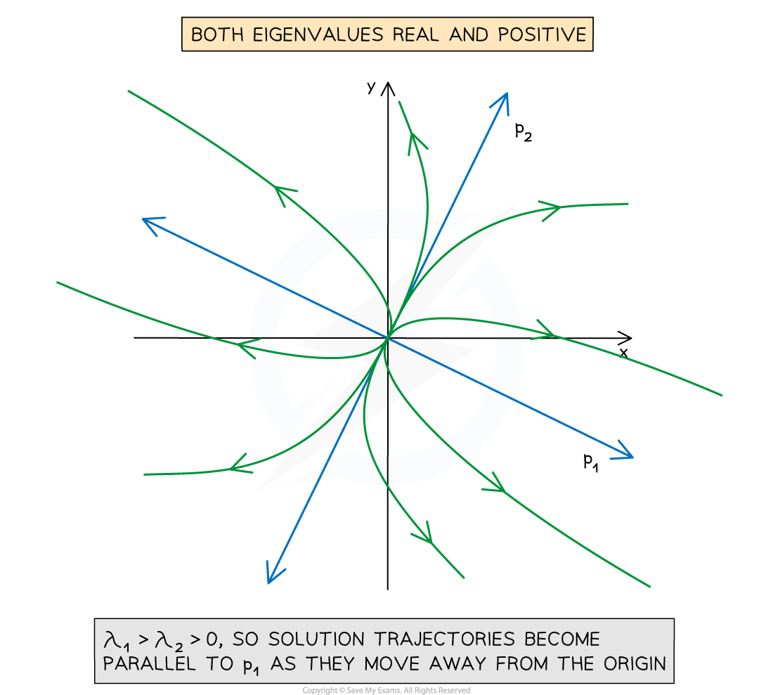
Both eigenvalues are positive
Suppose
format('truetype')%3Bfont-weight%3Anormal%3Bfont-style%3Anormal%3B%7D%3C%2Fstyle%3E%3C%2Fdefs%3E%3Ctext%20font-family%3D%22Times%20New%20Roman%22%20font-size%3D%2218%22%20font-style%3D%22italic%22%20text-anchor%3D%22middle%22%20x%3D%224.5%22%20y%3D%2216%22%3E%26%23x3BB%3B%3C%2Ftext%3E%3Ctext%20font-family%3D%22Times%20New%20Roman%22%20font-size%3D%2213%22%20text-anchor%3D%22middle%22%20x%3D%2213.5%22%20y%3D%2224%22%3E1%3C%2Ftext%3E%3Ctext%20font-family%3D%22math144f683a84163b3523afe57c2e0%22%20font-size%3D%2216%22%20text-anchor%3D%22middle%22%20x%3D%2225.5%22%20y%3D%2216%22%3E%26gt%3B%3C%2Ftext%3E%3Ctext%20font-family%3D%22Times%20New%20Roman%22%20font-size%3D%2218%22%20font-style%3D%22italic%22%20text-anchor%3D%22middle%22%20x%3D%2237.5%22%20y%3D%2216%22%3E%26%23x3BB%3B%3C%2Ftext%3E%3Ctext%20font-family%3D%22Times%20New%20Roman%22%20font-size%3D%2213%22%20text-anchor%3D%22middle%22%20x%3D%2246.5%22%20y%3D%2224%22%3E2%3C%2Ftext%3E%3Ctext%20font-family%3D%22math144f683a84163b3523afe57c2e0%22%20font-size%3D%2216%22%20text-anchor%3D%22middle%22%20x%3D%2258.5%22%20y%3D%2216%22%3E%26gt%3B%3C%2Ftext%3E%3Ctext%20font-family%3D%22Times%20New%20Roman%22%20font-size%3D%2218%22%20text-anchor%3D%22middle%22%20x%3D%2270.5%22%20y%3D%2216%22%3E0%3C%2Ftext%3E%3C%2Fsvg%3E)
All solution trajectories are directed away from the origin as t increases
To draw a solution trajectory
Start at the origin
Draw a line roughly parallel to
Move away from the origin and
Draw a line roughly parallel to
The line does not end
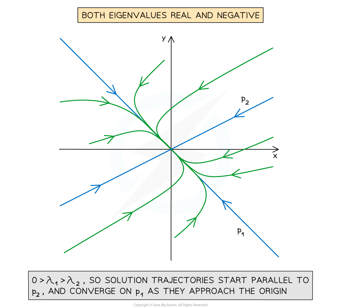
Both eigenvalues are negative
Suppose
format('truetype')%3Bfont-weight%3Anormal%3Bfont-style%3Anormal%3B%7D%3C%2Fstyle%3E%3C%2Fdefs%3E%3Ctext%20font-family%3D%22Times%20New%20Roman%22%20font-size%3D%2218%22%20text-anchor%3D%22middle%22%20x%3D%224.5%22%20y%3D%2216%22%3E0%3C%2Ftext%3E%3Ctext%20font-family%3D%22math144f683a84163b3523afe57c2e0%22%20font-size%3D%2216%22%20text-anchor%3D%22middle%22%20x%3D%2217.5%22%20y%3D%2216%22%3E%26gt%3B%3C%2Ftext%3E%3Ctext%20font-family%3D%22Times%20New%20Roman%22%20font-size%3D%2218%22%20font-style%3D%22italic%22%20text-anchor%3D%22middle%22%20x%3D%2229.5%22%20y%3D%2216%22%3E%26%23x3BB%3B%3C%2Ftext%3E%3Ctext%20font-family%3D%22Times%20New%20Roman%22%20font-size%3D%2213%22%20text-anchor%3D%22middle%22%20x%3D%2238.5%22%20y%3D%2224%22%3E1%3C%2Ftext%3E%3Ctext%20font-family%3D%22math144f683a84163b3523afe57c2e0%22%20font-size%3D%2216%22%20text-anchor%3D%22middle%22%20x%3D%2250.5%22%20y%3D%2216%22%3E%26gt%3B%3C%2Ftext%3E%3Ctext%20font-family%3D%22Times%20New%20Roman%22%20font-size%3D%2218%22%20font-style%3D%22italic%22%20text-anchor%3D%22middle%22%20x%3D%2262.5%22%20y%3D%2216%22%3E%26%23x3BB%3B%3C%2Ftext%3E%3Ctext%20font-family%3D%22Times%20New%20Roman%22%20font-size%3D%2213%22%20text-anchor%3D%22middle%22%20x%3D%2271.5%22%20y%3D%2224%22%3E2%3C%2Ftext%3E%3C%2Fsvg%3E)
All solution trajectories are directed towards the origin as t increases
To draw a solution trajectory
Start from somewhere at the edge of the graph
Draw a line roughly parallel to
Move toward the origin and away from
Draw a line roughly parallel to
End at the origin
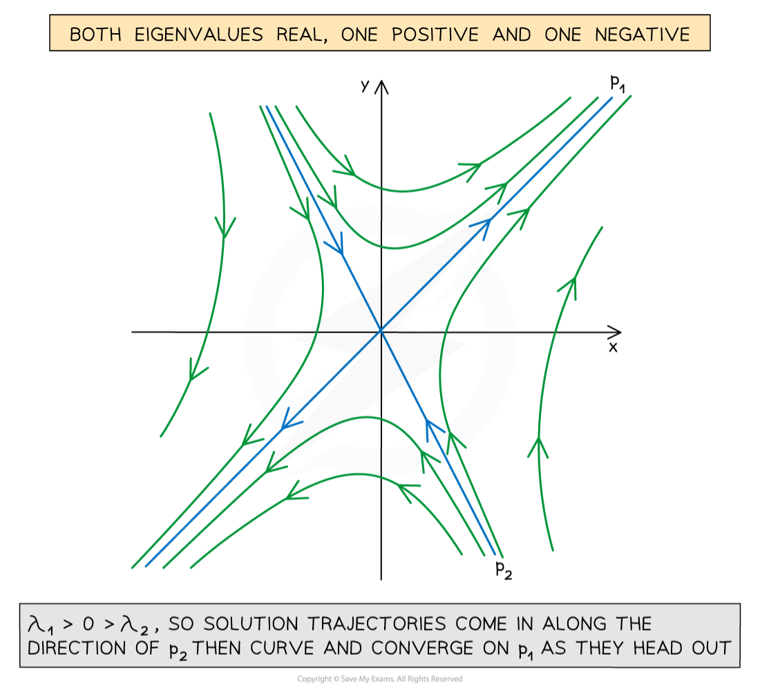
One positive and one negative eigenvalue
Suppose
format('truetype')%3Bfont-weight%3Anormal%3Bfont-style%3Anormal%3B%7D%3C%2Fstyle%3E%3C%2Fdefs%3E%3Ctext%20font-family%3D%22Times%20New%20Roman%22%20font-size%3D%2218%22%20font-style%3D%22italic%22%20text-anchor%3D%22middle%22%20x%3D%224.5%22%20y%3D%2216%22%3E%26%23x3BB%3B%3C%2Ftext%3E%3Ctext%20font-family%3D%22Times%20New%20Roman%22%20font-size%3D%2213%22%20text-anchor%3D%22middle%22%20x%3D%2213.5%22%20y%3D%2224%22%3E1%3C%2Ftext%3E%3Ctext%20font-family%3D%22math144f683a84163b3523afe57c2e0%22%20font-size%3D%2216%22%20text-anchor%3D%22middle%22%20x%3D%2225.5%22%20y%3D%2216%22%3E%26gt%3B%3C%2Ftext%3E%3Ctext%20font-family%3D%22Times%20New%20Roman%22%20font-size%3D%2218%22%20text-anchor%3D%22middle%22%20x%3D%2237.5%22%20y%3D%2216%22%3E0%3C%2Ftext%3E%3Ctext%20font-family%3D%22math144f683a84163b3523afe57c2e0%22%20font-size%3D%2216%22%20text-anchor%3D%22middle%22%20x%3D%2250.5%22%20y%3D%2216%22%3E%26gt%3B%3C%2Ftext%3E%3Ctext%20font-family%3D%22Times%20New%20Roman%22%20font-size%3D%2218%22%20font-style%3D%22italic%22%20text-anchor%3D%22middle%22%20x%3D%2262.5%22%20y%3D%2216%22%3E%26%23x3BB%3B%3C%2Ftext%3E%3Ctext%20font-family%3D%22Times%20New%20Roman%22%20font-size%3D%2213%22%20text-anchor%3D%22middle%22%20x%3D%2271.5%22%20y%3D%2224%22%3E2%3C%2Ftext%3E%3C%2Fsvg%3E)
To draw a solution trajectory
Start from somewhere at the edge of the graph
Draw a line roughly parallel to
Move toward the origin and away from
Move away from the origin and toward
Draw a line roughly parallel to
The line does not end
What does the phase portrait look like when the eigenvalues are complex numbers?
The phase portraits when the eigenvalues are complex always include curves orbiting the origin
They could be closed ellipses
They could be open spirals
The real part of the complex eigenvalues affect the shape
Positive real parts cause the trajectories to spiral away from the origin
Negative real parts cause the trajectories to spiral towards the origin
Zero real parts cause the trajectories to form ellipses centred at the origin
You can find the orientation of the trajectory by finding the value of
format('truetype')%3Bfont-weight%3Anormal%3Bfont-style%3Anormal%3B%7D%40font-face%7Bfont-family%3A'brack_sm2882ad605b1e27be87c7468'%3Bsrc%3Aurl(data%3Afont%2Ftruetype%3Bcharset%3Dutf-8%3Bbase64%2CAAEAAAAMAIAAAwBAT1MvMi7PH4UAAADMAAAATmNtYXA3kjw6AAABHAAAADxjdnQgAQYDiAAAAVgAAAASZ2x5ZkyYQ7YAAAFsAAAAkWhlYWQLyR8fAAACAAAAADZoaGVhAq0XCAAAAjgAAAAkaG10eDEjA%2FUAAAJcAAAADGxvY2EAAEKZAAACaAAAABBtYXhwBJsEcQAAAngAAAAgbmFtZW7QvZAAAAKYAAAB5XBvc3QArQBVAAAEgAAAACBwcmVwu5WEAAAABKAAAAAHAAACDAGQAAUAAAQABAAAAAAABAAEAAAAAAAAAQEAAAAAAAAAAAAAAAAAAAAAAAAAAAAAAAAAAAAAACAgICAAAAAg9AMD%2FP%2F8AAABVAABAAAAAAACAAEAAQAAABQAAwABAAAAFAAEACgAAAAGAAQAAQACI5wjn%2F%2F%2FAAAjnCOf%2F%2F%2FcZdxjAAEAAAAAAAAAAAFUAFQBAAArAIwAgACoAAcAAAACAAAAAADVAQEAAwAHAAAxMxEjFyM1M9XVq4CAAQHWqwABAAAAAABVAVgAAwAfGAGwAy%2BwADyxAgL1sAE8ALEDAD%2BwAjx8sQAG9bABPBEzESNVVQFY%2FqgAAQDXAAABLAFUAAMAIBgBsAUvsAE8sAI8sQAC9bADPACwAy%2BwAjyxAAH1sAE8EzMRI9dVVQFU%2FqwAAAAAAQAAAAEAAIsesexfDzz1AAMEAP%2F%2F%2F%2F%2FVre5k%2F%2F%2F%2F%2F9Wt7mT%2FgP%2F%2FAdYBWAAAAAoAAgABAAAAAAABAAABVP%2F%2FAAAXcP%2BA%2F4AB1gABAAAAAAAAAAAAAAAAAAAAAwDVAAABLAAAASwA1wAAAAAAAAAhAAAAWAAAAJEAAQAAAAMACgACAAAAAAACAIAEAAAAAAAEAABlAAAAAAAAABUBAgAAAAAAAAABACYAAAAAAAAAAAACAA4AJgAAAAAAAAADAEQANAAAAAAAAAAEACYAeAAAAAAAAAAFABYAngAAAAAAAAAGABMAtAAAAAAAAAAIABwAxwABAAAAAAABACYAAAABAAAAAAACAA4AJgABAAAAAAADAEQANAABAAAAAAAEACYAeAABAAAAAAAFABYAngABAAAAAAAGABMAtAABAAAAAAAIABwAxwADAAEECQABACYAAAADAAEECQACAA4AJgADAAEECQADAEQANAADAAEECQAEACYAeAADAAEECQAFABYAngADAAEECQAGABMAtAADAAEECQAIABwAxwBCAHIAYQBjAGsAZQB0AHMAIABzAG0AYQBsAGwAIABzAGkAegBlAFIAZQBnAHUAbABhAHIATQBhAHQAaABzACAARgBvAHIAIABNAG8AcgBlACAAQgByAGEAYwBrAGUAdABzACAAcwBtAGEAbABsACAAcwBpAHoAZQBCAHIAYQBjAGsAZQB0AHMAIABzAG0AYQBsAGwAIABzAGkAegBlAFYAZQByAHMAaQBvAG4AIAAyAC4AMEJyYWNrZXRzX3NtYWxsX3NpemUATQBhAHQAaABzACAARgBvAHIAIABNAG8AcgBlAAAAAAMAAAAAAAAAqgBVAAAAAAAAAAAAAAAAAAAAAAAAAAC5B%2F8AAo2FAA%3D%3D)format('truetype')%3Bfont-weight%3Anormal%3Bfont-style%3Anormal%3B%7D%40font-face%7Bfont-family%3A'bracketse552f5417ff4680c6b50499'%3Bsrc%3Aurl(data%3Afont%2Ftruetype%3Bcharset%3Dutf-8%3Bbase64%2CAAEAAAAMAIAAAwBAT1MvMi7RIisAAADMAAAATmNtYXBi7uzYAAABHAAAAExjdnQgBAkDLgAAAWgAAAASZ2x5Zo64f%2BkAAAF8AAABSWhlYWQLniGcAAACyAAAADZoaGVhBK4XLAAAAwAAAAAkaG10eCWq%2F90AAAMkAAAAFGxvY2EAABknAAADOAAAABhtYXhwBJIESAAAA1AAAAAgbmFtZRAA8I4AAANwAAAB3nBvc3QBwwDgAAAFUAAAACBwcmVwupWEAAAABXAAAAAHAAACggGQAAUAAAQABAAAAAAABAAEAAAAAAAAAQEAAAAAAAAAAAAAAAAAAAAAAAAAAAAAAAAAAAAAACAgICAAAAAg9AMEAAAAAAADgAAAAAAAAAACAAEAAQAAABQAAwABAAAAFAAEADgAAAAKAAgAAgACI5sjnSOeI6D%2F%2FwAAI5sjnSOeI6D%2F%2F9xm3GXcZdxkAAEAAAAAAAAAAAAAAAABVABWAQAALACoA4AAMgAHAAAAAgAAACoA1QNVAAMABwAANTMRIxMjETPV1auAgCoDK%2F0AAtUAAQAAAAABgAOAAAUAJBgBsAAvsAPFsQEC%2FbADELEEBP0AsQAAP7ABPLEEBj%2BwAzwwMTEzEAEjAFUBKyv%2BqwH8AYT%2BqgABAAAAAAGAA4AABQAmGAGwAC6wA8WxBQL9sAMQsQIE%2FQB8sQAGPxiwBTyxAwb2sAI8MDEREgEzABMBAVQr%2FtMCA4D91v6qAYQB%2FAAB%2F6wAAAEsA4AABQAnGAGwAC%2BwBzywA8WxAQL9sAMQsQQE%2FQCxAAA%2FsAE8sQQGP7ADPDAxISMSATMAASxVAf7UKwFVAfwBhP6rAAH%2FrAAAASwDgAAFACkYAbABL7AHPLAExbEAAv2wBBCxAwT9AHyxAQY%2FsAA8GLEEAD%2BwAzwwMRMzEAEjANdV%2FqsrASsDgP3V%2FqsBhgAAAAABAAAAAQAAeuTcpl8PPPUAAwQA%2F%2F%2F%2F%2F9Wt7o7%2F%2F%2F%2F%2F1a3ujv%2BsAAABgAOAAAAACgACAAEAAAAAAAEAAAOAAAAAABdw%2F6z%2FrAGAAAEAAAAAAAAAAAAAAAAAAAAFANUAAAEsAAABLAAAASz%2FrAEs%2F6wAAAAAAAAAJAAAAGgAAACzAAAA%2FQAAAUkAAQAAAAUACAACAAAAAAACAIAEAAAAAAAEAAA%2BAAAAAAAAABUBAgAAAAAAAAABACQAAAAAAAAAAAACAA4AJAAAAAAAAAADAEIAMgAAAAAAAAAEACQAdAAAAAAAAAAFABYAmAAAAAAAAAAGABIArgAAAAAAAAAIABwAwAABAAAAAAABACQAAAABAAAAAAACAA4AJAABAAAAAAADAEIAMgABAAAAAAAEACQAdAABAAAAAAAFABYAmAABAAAAAAAGABIArgABAAAAAAAIABwAwAADAAEECQABACQAAAADAAEECQACAA4AJAADAAEECQADAEIAMgADAAEECQAEACQAdAADAAEECQAFABYAmAADAAEECQAGABIArgADAAEECQAIABwAwABCAHIAYQBjAGsAZQB0AHMAIABmAHUAbABsACAAcwBpAHoAZQBSAGUAZwB1AGwAYQByAE0AYQB0AGgAcwAgAEYAbwByACAATQBvAHIAZQAgAEIAcgBhAGMAawBlAHQAcwAgAGYAdQBsAGwAIABzAGkAegBlAEIAcgBhAGMAawBlAHQAcwAgAGYAdQBsAGwAIABzAGkAegBlAFYAZQByAHMAaQBvAG4AIAAyAC4AMEJyYWNrZXRzX2Z1bGxfc2l6ZQBNAGEAdABoAHMAIABGAG8AcgAgAE0AbwByAGUAAAADAAAAAAAAAcAA4AAAAAAAAAAAAAAAAAAAAAAAAAAAuQf%2FAAGNhQA%3D)format('truetype')%3Bfont-weight%3Anormal%3Bfont-style%3Anormal%3B%7D%3C%2Fstyle%3E%3C%2Fdefs%3E%3Ctext%20font-family%3D%22bracketse552f5417ff4680c6b50499%22%20font-size%3D%2218%22%20text-anchor%3D%22start%22%20x%3D%221.5%22%20y%3D%2217%22%3E%26%23x239B%3B%3C%2Ftext%3E%3Ctext%20font-family%3D%22brack_sm2882ad605b1e27be87c7468%22%20font-size%3D%2218%22%20text-anchor%3D%22start%22%20x%3D%221.5%22%20y%3D%2223%22%3E%26%23x239C%3B%3C%2Ftext%3E%3Ctext%20font-family%3D%22brack_sm2882ad605b1e27be87c7468%22%20font-size%3D%2218%22%20text-anchor%3D%22start%22%20x%3D%221.5%22%20y%3D%2229%22%3E%26%23x239C%3B%3C%2Ftext%3E%3Ctext%20font-family%3D%22brack_sm2882ad605b1e27be87c7468%22%20font-size%3D%2218%22%20text-anchor%3D%22start%22%20x%3D%221.5%22%20y%3D%2235%22%3E%26%23x239C%3B%3C%2Ftext%3E%3Ctext%20font-family%3D%22brack_sm2882ad605b1e27be87c7468%22%20font-size%3D%2218%22%20text-anchor%3D%22start%22%20x%3D%221.5%22%20y%3D%2241%22%3E%26%23x239C%3B%3C%2Ftext%3E%3Ctext%20font-family%3D%22bracketse552f5417ff4680c6b50499%22%20font-size%3D%2218%22%20text-anchor%3D%22start%22%20x%3D%221.5%22%20y%3D%2257%22%3E%26%23x239D%3B%3C%2Ftext%3E%3Ctext%20font-family%3D%22bracketse552f5417ff4680c6b50499%22%20font-size%3D%2218%22%20text-anchor%3D%22start%22%20x%3D%2226.5%22%20y%3D%2217%22%3E%26%23x239E%3B%3C%2Ftext%3E%3Ctext%20font-family%3D%22brack_sm2882ad605b1e27be87c7468%22%20font-size%3D%2218%22%20text-anchor%3D%22start%22%20x%3D%2226.5%22%20y%3D%2223%22%3E%26%23x239F%3B%3C%2Ftext%3E%3Ctext%20font-family%3D%22brack_sm2882ad605b1e27be87c7468%22%20font-size%3D%2218%22%20text-anchor%3D%22start%22%20x%3D%2226.5%22%20y%3D%2229%22%3E%26%23x239F%3B%3C%2Ftext%3E%3Ctext%20font-family%3D%22brack_sm2882ad605b1e27be87c7468%22%20font-size%3D%2218%22%20text-anchor%3D%22start%22%20x%3D%2226.5%22%20y%3D%2235%22%3E%26%23x239F%3B%3C%2Ftext%3E%3Ctext%20font-family%3D%22brack_sm2882ad605b1e27be87c7468%22%20font-size%3D%2218%22%20text-anchor%3D%22start%22%20x%3D%2226.5%22%20y%3D%2241%22%3E%26%23x239F%3B%3C%2Ftext%3E%3Ctext%20font-family%3D%22bracketse552f5417ff4680c6b50499%22%20font-size%3D%2218%22%20text-anchor%3D%22start%22%20x%3D%2226.5%22%20y%3D%2257%22%3E%26%23x23A0%3B%3C%2Ftext%3E%3Ctext%20font-family%3D%22math1d9d4f495e875a2e075a1a4a6e1%22%20font-size%3D%2212%22%20text-anchor%3D%22middle%22%20x%3D%2216.5%22%20y%3D%2210%22%3E.%3C%2Ftext%3E%3Ctext%20font-family%3D%22Times%20New%20Roman%22%20font-size%3D%2218%22%20font-style%3D%22italic%22%20text-anchor%3D%22middle%22%20x%3D%2215.5%22%20y%3D%2221%22%3Ex%3C%2Ftext%3E%3Ctext%20font-family%3D%22math1d9d4f495e875a2e075a1a4a6e1%22%20font-size%3D%2212%22%20text-anchor%3D%22middle%22%20x%3D%2216.5%22%20y%3D%2238%22%3E.%3C%2Ftext%3E%3Ctext%20font-family%3D%22Times%20New%20Roman%22%20font-size%3D%2218%22%20font-style%3D%22italic%22%20text-anchor%3D%22middle%22%20x%3D%2215.5%22%20y%3D%2249%22%3Ey%3C%2Ftext%3E%3C%2Fsvg%3E) at a specific point on one of the coordinate axes
at a specific point on one of the coordinate axesFor example, consider the system
format('truetype')%3Bfont-weight%3Anormal%3Bfont-style%3Anormal%3B%7D%40font-face%7Bfont-family%3A'brack_sm2882ad605b1e27be87c7468'%3Bsrc%3Aurl(data%3Afont%2Ftruetype%3Bcharset%3Dutf-8%3Bbase64%2CAAEAAAAMAIAAAwBAT1MvMi7PH4UAAADMAAAATmNtYXA3kjw6AAABHAAAADxjdnQgAQYDiAAAAVgAAAASZ2x5ZkyYQ7YAAAFsAAAAkWhlYWQLyR8fAAACAAAAADZoaGVhAq0XCAAAAjgAAAAkaG10eDEjA%2FUAAAJcAAAADGxvY2EAAEKZAAACaAAAABBtYXhwBJsEcQAAAngAAAAgbmFtZW7QvZAAAAKYAAAB5XBvc3QArQBVAAAEgAAAACBwcmVwu5WEAAAABKAAAAAHAAACDAGQAAUAAAQABAAAAAAABAAEAAAAAAAAAQEAAAAAAAAAAAAAAAAAAAAAAAAAAAAAAAAAAAAAACAgICAAAAAg9AMD%2FP%2F8AAABVAABAAAAAAACAAEAAQAAABQAAwABAAAAFAAEACgAAAAGAAQAAQACI5wjn%2F%2F%2FAAAjnCOf%2F%2F%2FcZdxjAAEAAAAAAAAAAAFUAFQBAAArAIwAgACoAAcAAAACAAAAAADVAQEAAwAHAAAxMxEjFyM1M9XVq4CAAQHWqwABAAAAAABVAVgAAwAfGAGwAy%2BwADyxAgL1sAE8ALEDAD%2BwAjx8sQAG9bABPBEzESNVVQFY%2FqgAAQDXAAABLAFUAAMAIBgBsAUvsAE8sAI8sQAC9bADPACwAy%2BwAjyxAAH1sAE8EzMRI9dVVQFU%2FqwAAAAAAQAAAAEAAIsesexfDzz1AAMEAP%2F%2F%2F%2F%2FVre5k%2F%2F%2F%2F%2F9Wt7mT%2FgP%2F%2FAdYBWAAAAAoAAgABAAAAAAABAAABVP%2F%2FAAAXcP%2BA%2F4AB1gABAAAAAAAAAAAAAAAAAAAAAwDVAAABLAAAASwA1wAAAAAAAAAhAAAAWAAAAJEAAQAAAAMACgACAAAAAAACAIAEAAAAAAAEAABlAAAAAAAAABUBAgAAAAAAAAABACYAAAAAAAAAAAACAA4AJgAAAAAAAAADAEQANAAAAAAAAAAEACYAeAAAAAAAAAAFABYAngAAAAAAAAAGABMAtAAAAAAAAAAIABwAxwABAAAAAAABACYAAAABAAAAAAACAA4AJgABAAAAAAADAEQANAABAAAAAAAEACYAeAABAAAAAAAFABYAngABAAAAAAAGABMAtAABAAAAAAAIABwAxwADAAEECQABACYAAAADAAEECQACAA4AJgADAAEECQADAEQANAADAAEECQAEACYAeAADAAEECQAFABYAngADAAEECQAGABMAtAADAAEECQAIABwAxwBCAHIAYQBjAGsAZQB0AHMAIABzAG0AYQBsAGwAIABzAGkAegBlAFIAZQBnAHUAbABhAHIATQBhAHQAaABzACAARgBvAHIAIABNAG8AcgBlACAAQgByAGEAYwBrAGUAdABzACAAcwBtAGEAbABsACAAcwBpAHoAZQBCAHIAYQBjAGsAZQB0AHMAIABzAG0AYQBsAGwAIABzAGkAegBlAFYAZQByAHMAaQBvAG4AIAAyAC4AMEJyYWNrZXRzX3NtYWxsX3NpemUATQBhAHQAaABzACAARgBvAHIAIABNAG8AcgBlAAAAAAMAAAAAAAAAqgBVAAAAAAAAAAAAAAAAAAAAAAAAAAC5B%2F8AAo2FAA%3D%3D)format('truetype')%3Bfont-weight%3Anormal%3Bfont-style%3Anormal%3B%7D%40font-face%7Bfont-family%3A'bracketse552f5417ff4680c6b50499'%3Bsrc%3Aurl(data%3Afont%2Ftruetype%3Bcharset%3Dutf-8%3Bbase64%2CAAEAAAAMAIAAAwBAT1MvMi7RIisAAADMAAAATmNtYXBi7uzYAAABHAAAAExjdnQgBAkDLgAAAWgAAAASZ2x5Zo64f%2BkAAAF8AAABSWhlYWQLniGcAAACyAAAADZoaGVhBK4XLAAAAwAAAAAkaG10eCWq%2F90AAAMkAAAAFGxvY2EAABknAAADOAAAABhtYXhwBJIESAAAA1AAAAAgbmFtZRAA8I4AAANwAAAB3nBvc3QBwwDgAAAFUAAAACBwcmVwupWEAAAABXAAAAAHAAACggGQAAUAAAQABAAAAAAABAAEAAAAAAAAAQEAAAAAAAAAAAAAAAAAAAAAAAAAAAAAAAAAAAAAACAgICAAAAAg9AMEAAAAAAADgAAAAAAAAAACAAEAAQAAABQAAwABAAAAFAAEADgAAAAKAAgAAgACI5sjnSOeI6D%2F%2FwAAI5sjnSOeI6D%2F%2F9xm3GXcZdxkAAEAAAAAAAAAAAAAAAABVABWAQAALACoA4AAMgAHAAAAAgAAACoA1QNVAAMABwAANTMRIxMjETPV1auAgCoDK%2F0AAtUAAQAAAAABgAOAAAUAJBgBsAAvsAPFsQEC%2FbADELEEBP0AsQAAP7ABPLEEBj%2BwAzwwMTEzEAEjAFUBKyv%2BqwH8AYT%2BqgABAAAAAAGAA4AABQAmGAGwAC6wA8WxBQL9sAMQsQIE%2FQB8sQAGPxiwBTyxAwb2sAI8MDEREgEzABMBAVQr%2FtMCA4D91v6qAYQB%2FAAB%2F6wAAAEsA4AABQAnGAGwAC%2BwBzywA8WxAQL9sAMQsQQE%2FQCxAAA%2FsAE8sQQGP7ADPDAxISMSATMAASxVAf7UKwFVAfwBhP6rAAH%2FrAAAASwDgAAFACkYAbABL7AHPLAExbEAAv2wBBCxAwT9AHyxAQY%2FsAA8GLEEAD%2BwAzwwMRMzEAEjANdV%2FqsrASsDgP3V%2FqsBhgAAAAABAAAAAQAAeuTcpl8PPPUAAwQA%2F%2F%2F%2F%2F9Wt7o7%2F%2F%2F%2F%2F1a3ujv%2BsAAABgAOAAAAACgACAAEAAAAAAAEAAAOAAAAAABdw%2F6z%2FrAGAAAEAAAAAAAAAAAAAAAAAAAAFANUAAAEsAAABLAAAASz%2FrAEs%2F6wAAAAAAAAAJAAAAGgAAACzAAAA%2FQAAAUkAAQAAAAUACAACAAAAAAACAIAEAAAAAAAEAAA%2BAAAAAAAAABUBAgAAAAAAAAABACQAAAAAAAAAAAACAA4AJAAAAAAAAAADAEIAMgAAAAAAAAAEACQAdAAAAAAAAAAFABYAmAAAAAAAAAAGABIArgAAAAAAAAAIABwAwAABAAAAAAABACQAAAABAAAAAAACAA4AJAABAAAAAAADAEIAMgABAAAAAAAEACQAdAABAAAAAAAFABYAmAABAAAAAAAGABIArgABAAAAAAAIABwAwAADAAEECQABACQAAAADAAEECQACAA4AJAADAAEECQADAEIAMgADAAEECQAEACQAdAADAAEECQAFABYAmAADAAEECQAGABIArgADAAEECQAIABwAwABCAHIAYQBjAGsAZQB0AHMAIABmAHUAbABsACAAcwBpAHoAZQBSAGUAZwB1AGwAYQByAE0AYQB0AGgAcwAgAEYAbwByACAATQBvAHIAZQAgAEIAcgBhAGMAawBlAHQAcwAgAGYAdQBsAGwAIABzAGkAegBlAEIAcgBhAGMAawBlAHQAcwAgAGYAdQBsAGwAIABzAGkAegBlAFYAZQByAHMAaQBvAG4AIAAyAC4AMEJyYWNrZXRzX2Z1bGxfc2l6ZQBNAGEAdABoAHMAIABGAG8AcgAgAE0AbwByAGUAAAADAAAAAAAAAcAA4AAAAAAAAAAAAAAAAAAAAAAAAAAAuQf%2FAAGNhQA%3D)format('truetype')%3Bfont-weight%3Anormal%3Bfont-style%3Anormal%3B%7D%3C%2Fstyle%3E%3C%2Fdefs%3E%3Ctext%20font-family%3D%22math16d8888858ea6f9ebce8ea398ff%22%20font-size%3D%2212%22%20font-weight%3D%22bold%22%20text-anchor%3D%22middle%22%20x%3D%225.5%22%20y%3D%2221%22%3E.%3C%2Ftext%3E%3Ctext%20font-family%3D%22Times%20New%20Roman%22%20font-size%3D%2218%22%20font-style%3D%22italic%22%20font-weight%3D%22bold%22%20text-anchor%3D%22middle%22%20x%3D%225.5%22%20y%3D%2233%22%3Ex%3C%2Ftext%3E%3Ctext%20font-family%3D%22math16d8888858ea6f9ebce8ea398ff%22%20font-size%3D%2216%22%20text-anchor%3D%22middle%22%20x%3D%2219.5%22%20y%3D%2233%22%3E%3D%3C%2Ftext%3E%3Ctext%20font-family%3D%22bracketse552f5417ff4680c6b50499%22%20font-size%3D%2218%22%20text-anchor%3D%22start%22%20x%3D%2229.5%22%20y%3D%2218%22%3E%26%23x239B%3B%3C%2Ftext%3E%3Ctext%20font-family%3D%22brack_sm2882ad605b1e27be87c7468%22%20font-size%3D%2218%22%20text-anchor%3D%22start%22%20x%3D%2229.5%22%20y%3D%2224%22%3E%26%23x239C%3B%3C%2Ftext%3E%3Ctext%20font-family%3D%22brack_sm2882ad605b1e27be87c7468%22%20font-size%3D%2218%22%20text-anchor%3D%22start%22%20x%3D%2229.5%22%20y%3D%2230%22%3E%26%23x239C%3B%3C%2Ftext%3E%3Ctext%20font-family%3D%22brack_sm2882ad605b1e27be87c7468%22%20font-size%3D%2218%22%20text-anchor%3D%22start%22%20x%3D%2229.5%22%20y%3D%2236%22%3E%26%23x239C%3B%3C%2Ftext%3E%3Ctext%20font-family%3D%22bracketse552f5417ff4680c6b50499%22%20font-size%3D%2218%22%20text-anchor%3D%22start%22%20x%3D%2229.5%22%20y%3D%2252%22%3E%26%23x239D%3B%3C%2Ftext%3E%3Ctext%20font-family%3D%22bracketse552f5417ff4680c6b50499%22%20font-size%3D%2218%22%20text-anchor%3D%22start%22%20x%3D%2283.5%22%20y%3D%2218%22%3E%26%23x239E%3B%3C%2Ftext%3E%3Ctext%20font-family%3D%22brack_sm2882ad605b1e27be87c7468%22%20font-size%3D%2218%22%20text-anchor%3D%22start%22%20x%3D%2283.5%22%20y%3D%2224%22%3E%26%23x239F%3B%3C%2Ftext%3E%3Ctext%20font-family%3D%22brack_sm2882ad605b1e27be87c7468%22%20font-size%3D%2218%22%20text-anchor%3D%22start%22%20x%3D%2283.5%22%20y%3D%2230%22%3E%26%23x239F%3B%3C%2Ftext%3E%3Ctext%20font-family%3D%22brack_sm2882ad605b1e27be87c7468%22%20font-size%3D%2218%22%20text-anchor%3D%22start%22%20x%3D%2283.5%22%20y%3D%2236%22%3E%26%23x239F%3B%3C%2Ftext%3E%3Ctext%20font-family%3D%22bracketse552f5417ff4680c6b50499%22%20font-size%3D%2218%22%20text-anchor%3D%22start%22%20x%3D%2283.5%22%20y%3D%2252%22%3E%26%23x23A0%3B%3C%2Ftext%3E%3Ctext%20font-family%3D%22Times%20New%20Roman%22%20font-size%3D%2218%22%20text-anchor%3D%22middle%22%20x%3D%2243.5%22%20y%3D%2219%22%3E1%3C%2Ftext%3E%3Ctext%20font-family%3D%22math16d8888858ea6f9ebce8ea398ff%22%20font-size%3D%2216%22%20text-anchor%3D%22middle%22%20x%3D%2262.5%22%20y%3D%2219%22%3E%26%23x2212%3B%3C%2Ftext%3E%3Ctext%20font-family%3D%22Times%20New%20Roman%22%20font-size%3D%2218%22%20text-anchor%3D%22middle%22%20x%3D%2273.5%22%20y%3D%2219%22%3E2%3C%2Ftext%3E%3Ctext%20font-family%3D%22Times%20New%20Roman%22%20font-size%3D%2218%22%20text-anchor%3D%22middle%22%20x%3D%2243.5%22%20y%3D%2245%22%3E1%3C%2Ftext%3E%3Ctext%20font-family%3D%22math16d8888858ea6f9ebce8ea398ff%22%20font-size%3D%2216%22%20text-anchor%3D%22middle%22%20x%3D%2262.5%22%20y%3D%2245%22%3E%26%23x2212%3B%3C%2Ftext%3E%3Ctext%20font-family%3D%22Times%20New%20Roman%22%20font-size%3D%2218%22%20text-anchor%3D%22middle%22%20x%3D%2273.5%22%20y%3D%2245%22%3E1%3C%2Ftext%3E%3Ctext%20font-family%3D%22Times%20New%20Roman%22%20font-size%3D%2218%22%20font-style%3D%22italic%22%20font-weight%3D%22bold%22%20text-anchor%3D%22middle%22%20x%3D%2294.5%22%20y%3D%2233%22%3Ex%3C%2Ftext%3E%3C%2Fsvg%3E)
Pick the point
format('truetype')%3Bfont-weight%3Anormal%3Bfont-style%3Anormal%3B%7D%40font-face%7Bfont-family%3A'round_brackets18549f92a457f2409'%3Bsrc%3Aurl(data%3Afont%2Ftruetype%3Bcharset%3Dutf-8%3Bbase64%2CAAEAAAAMAIAAAwBAT1MvMjwHLFQAAADMAAAATmNtYXDf7xCrAAABHAAAADxjdnQgBAkDLgAAAVgAAAASZ2x5ZmAOz2cAAAFsAAABJGhlYWQOKih8AAACkAAAADZoaGVhCvgVwgAAAsgAAAAkaG10eCA6AAIAAALsAAAADGxvY2EAAARLAAAC%2BAAAABBtYXhwBIgEWQAAAwgAAAAgbmFtZXHR30MAAAMoAAACOXBvc3QDogHPAAAFZAAAACBwcmVwupWEAAAABYQAAAAHAAAGcgGQAAUAAAgACAAAAAAACAAIAAAAAAAAAQIAAAAAAAAAAAAAAAAAAAAAAAAAAAAAAAAAAAAAACAgICAAAAAo8AMGe%2F57AAAHPgGyAAAAAAACAAEAAQAAABQAAwABAAAAFAAEACgAAAAGAAQAAQACACgAKf%2F%2FAAAAKAAp%2F%2F%2F%2F2f%2FZAAEAAAAAAAAAAAFUAFYBAAAsAKgDgAAyAAcAAAACAAAAKgDVA1UAAwAHAAA1MxEjEyMRM9XVq4CAKgMr%2FQAC1QABAAD%2B0AIgBtAACQBNGAGwChCwA9SwAxCwAtSwChCwBdSwBRCwANSwAxCwBzywAhCwCDwAsAoQsAPUsAMQsAfUsAoQsAXUsAoQsADUsAMQsAI8sAcQsAg8MTAREAEzABEQASMAAZCQ%2FnABkJD%2BcALQ%2FZD%2BcAGQAnACcAGQ%2FnAAAQAA%2FtACIAbQAAkATRgBsAoQsAPUsAMQsALUsAoQsAXUsAUQsADUsAMQsAc8sAIQsAg8ALAKELAD1LADELAH1LAKELAF1LAKELAA1LADELACPLAHELAIPDEwARABIwAREAEzAAIg%2FnCQAZD%2BcJABkALQ%2FZD%2BcAGQAnACcAGQ%2FnAAAQAAAAEAAPW2NYFfDzz1AAMIAP%2F%2F%2F%2F%2FVre7u%2F%2F%2F%2F%2F9Wt7u4AAP7QA7cG0AAAAAoAAgABAAAAAAABAAAHPv5OAAAXcAAA%2F%2F4DtwABAAAAAAAAAAAAAAAAAAAAAwDVAAACIAAAAiAAAAAAAAAAAAAkAAAAowAAASQAAQAAAAMACgACAAAAAAACAIAEAAAAAAAEAABNAAAAAAAAABUBAgAAAAAAAAABAD4AAAAAAAAAAAACAA4APgAAAAAAAAADAFwATAAAAAAAAAAEAD4AqAAAAAAAAAAFABYA5gAAAAAAAAAGAB8A%2FAAAAAAAAAAIABwBGwABAAAAAAABAD4AAAABAAAAAAACAA4APgABAAAAAAADAFwATAABAAAAAAAEAD4AqAABAAAAAAAFABYA5gABAAAAAAAGAB8A%2FAABAAAAAAAIABwBGwADAAEECQABAD4AAAADAAEECQACAA4APgADAAEECQADAFwATAADAAEECQAEAD4AqAADAAEECQAFABYA5gADAAEECQAGAB8A%2FAADAAEECQAIABwBGwBSAG8AdQBuAGQAIABiAHIAYQBjAGsAZQB0AHMAIAB3AGkAdABoACAAYQBzAGMAZQBuAHQAIAAxADgANQA0AFIAZQBnAHUAbABhAHIATQBhAHQAaABzACAARgBvAHIAIABNAG8AcgBlACAAUgBvAHUAbgBkACAAYgByAGEAYwBrAGUAdABzACAAdwBpAHQAaAAgAGEAcwBjAGUAbgB0ACAAMQA4ADUANABSAG8AdQBuAGQAIABiAHIAYQBjAGsAZQB0AHMAIAB3AGkAdABoACAAYQBzAGMAZQBuAHQAIAAxADgANQA0AFYAZQByAHMAaQBvAG4AIAAyAC4AMFJvdW5kX2JyYWNrZXRzX3dpdGhfYXNjZW50XzE4NTQATQBhAHQAaABzACAARgBvAHIAIABNAG8AcgBlAAAAAAMAAAAAAAADnwHPAAAAAAAAAAAAAAAAAAAAAAAAAAC5B%2F8AAY2FAA%3D%3D)format('truetype')%3Bfont-weight%3Anormal%3Bfont-style%3Anormal%3B%7D%3C%2Fstyle%3E%3C%2Fdefs%3E%3Ctext%20font-family%3D%22round_brackets18549f92a457f2409%22%20font-size%3D%2218%22%20text-anchor%3D%22middle%22%20x%3D%223.5%22%20y%3D%2216%22%3E(%3C%2Ftext%3E%3Ctext%20font-family%3D%22round_brackets18549f92a457f2409%22%20font-size%3D%2218%22%20text-anchor%3D%22middle%22%20x%3D%2235.5%22%20y%3D%2216%22%3E)%3C%2Ftext%3E%3Ctext%20font-family%3D%22Times%20New%20Roman%22%20font-size%3D%2218%22%20text-anchor%3D%22middle%22%20x%3D%2210.5%22%20y%3D%2216%22%3E1%3C%2Ftext%3E%3Ctext%20font-family%3D%22math1f7177163c833dff4b38fc8d287%22%20font-size%3D%2216%22%20text-anchor%3D%22middle%22%20x%3D%2217.5%22%20y%3D%2216%22%3E%2C%3C%2Ftext%3E%3Ctext%20font-family%3D%22Times%20New%20Roman%22%20font-size%3D%2218%22%20text-anchor%3D%22middle%22%20x%3D%2228.5%22%20y%3D%2216%22%3E0%3C%2Ftext%3E%3C%2Fsvg%3E)
format('truetype')%3Bfont-weight%3Anormal%3Bfont-style%3Anormal%3B%7D%40font-face%7Bfont-family%3A'brack_sm2882ad605b1e27be87c7468'%3Bsrc%3Aurl(data%3Afont%2Ftruetype%3Bcharset%3Dutf-8%3Bbase64%2CAAEAAAAMAIAAAwBAT1MvMi7PH4UAAADMAAAATmNtYXA3kjw6AAABHAAAADxjdnQgAQYDiAAAAVgAAAASZ2x5ZkyYQ7YAAAFsAAAAkWhlYWQLyR8fAAACAAAAADZoaGVhAq0XCAAAAjgAAAAkaG10eDEjA%2FUAAAJcAAAADGxvY2EAAEKZAAACaAAAABBtYXhwBJsEcQAAAngAAAAgbmFtZW7QvZAAAAKYAAAB5XBvc3QArQBVAAAEgAAAACBwcmVwu5WEAAAABKAAAAAHAAACDAGQAAUAAAQABAAAAAAABAAEAAAAAAAAAQEAAAAAAAAAAAAAAAAAAAAAAAAAAAAAAAAAAAAAACAgICAAAAAg9AMD%2FP%2F8AAABVAABAAAAAAACAAEAAQAAABQAAwABAAAAFAAEACgAAAAGAAQAAQACI5wjn%2F%2F%2FAAAjnCOf%2F%2F%2FcZdxjAAEAAAAAAAAAAAFUAFQBAAArAIwAgACoAAcAAAACAAAAAADVAQEAAwAHAAAxMxEjFyM1M9XVq4CAAQHWqwABAAAAAABVAVgAAwAfGAGwAy%2BwADyxAgL1sAE8ALEDAD%2BwAjx8sQAG9bABPBEzESNVVQFY%2FqgAAQDXAAABLAFUAAMAIBgBsAUvsAE8sAI8sQAC9bADPACwAy%2BwAjyxAAH1sAE8EzMRI9dVVQFU%2FqwAAAAAAQAAAAEAAIsesexfDzz1AAMEAP%2F%2F%2F%2F%2FVre5k%2F%2F%2F%2F%2F9Wt7mT%2FgP%2F%2FAdYBWAAAAAoAAgABAAAAAAABAAABVP%2F%2FAAAXcP%2BA%2F4AB1gABAAAAAAAAAAAAAAAAAAAAAwDVAAABLAAAASwA1wAAAAAAAAAhAAAAWAAAAJEAAQAAAAMACgACAAAAAAACAIAEAAAAAAAEAABlAAAAAAAAABUBAgAAAAAAAAABACYAAAAAAAAAAAACAA4AJgAAAAAAAAADAEQANAAAAAAAAAAEACYAeAAAAAAAAAAFABYAngAAAAAAAAAGABMAtAAAAAAAAAAIABwAxwABAAAAAAABACYAAAABAAAAAAACAA4AJgABAAAAAAADAEQANAABAAAAAAAEACYAeAABAAAAAAAFABYAngABAAAAAAAGABMAtAABAAAAAAAIABwAxwADAAEECQABACYAAAADAAEECQACAA4AJgADAAEECQADAEQANAADAAEECQAEACYAeAADAAEECQAFABYAngADAAEECQAGABMAtAADAAEECQAIABwAxwBCAHIAYQBjAGsAZQB0AHMAIABzAG0AYQBsAGwAIABzAGkAegBlAFIAZQBnAHUAbABhAHIATQBhAHQAaABzACAARgBvAHIAIABNAG8AcgBlACAAQgByAGEAYwBrAGUAdABzACAAcwBtAGEAbABsACAAcwBpAHoAZQBCAHIAYQBjAGsAZQB0AHMAIABzAG0AYQBsAGwAIABzAGkAegBlAFYAZQByAHMAaQBvAG4AIAAyAC4AMEJyYWNrZXRzX3NtYWxsX3NpemUATQBhAHQAaABzACAARgBvAHIAIABNAG8AcgBlAAAAAAMAAAAAAAAAqgBVAAAAAAAAAAAAAAAAAAAAAAAAAAC5B%2F8AAo2FAA%3D%3D)format('truetype')%3Bfont-weight%3Anormal%3Bfont-style%3Anormal%3B%7D%40font-face%7Bfont-family%3A'bracketse552f5417ff4680c6b50499'%3Bsrc%3Aurl(data%3Afont%2Ftruetype%3Bcharset%3Dutf-8%3Bbase64%2CAAEAAAAMAIAAAwBAT1MvMi7RIisAAADMAAAATmNtYXBi7uzYAAABHAAAAExjdnQgBAkDLgAAAWgAAAASZ2x5Zo64f%2BkAAAF8AAABSWhlYWQLniGcAAACyAAAADZoaGVhBK4XLAAAAwAAAAAkaG10eCWq%2F90AAAMkAAAAFGxvY2EAABknAAADOAAAABhtYXhwBJIESAAAA1AAAAAgbmFtZRAA8I4AAANwAAAB3nBvc3QBwwDgAAAFUAAAACBwcmVwupWEAAAABXAAAAAHAAACggGQAAUAAAQABAAAAAAABAAEAAAAAAAAAQEAAAAAAAAAAAAAAAAAAAAAAAAAAAAAAAAAAAAAACAgICAAAAAg9AMEAAAAAAADgAAAAAAAAAACAAEAAQAAABQAAwABAAAAFAAEADgAAAAKAAgAAgACI5sjnSOeI6D%2F%2FwAAI5sjnSOeI6D%2F%2F9xm3GXcZdxkAAEAAAAAAAAAAAAAAAABVABWAQAALACoA4AAMgAHAAAAAgAAACoA1QNVAAMABwAANTMRIxMjETPV1auAgCoDK%2F0AAtUAAQAAAAABgAOAAAUAJBgBsAAvsAPFsQEC%2FbADELEEBP0AsQAAP7ABPLEEBj%2BwAzwwMTEzEAEjAFUBKyv%2BqwH8AYT%2BqgABAAAAAAGAA4AABQAmGAGwAC6wA8WxBQL9sAMQsQIE%2FQB8sQAGPxiwBTyxAwb2sAI8MDEREgEzABMBAVQr%2FtMCA4D91v6qAYQB%2FAAB%2F6wAAAEsA4AABQAnGAGwAC%2BwBzywA8WxAQL9sAMQsQQE%2FQCxAAA%2FsAE8sQQGP7ADPDAxISMSATMAASxVAf7UKwFVAfwBhP6rAAH%2FrAAAASwDgAAFACkYAbABL7AHPLAExbEAAv2wBBCxAwT9AHyxAQY%2FsAA8GLEEAD%2BwAzwwMRMzEAEjANdV%2FqsrASsDgP3V%2FqsBhgAAAAABAAAAAQAAeuTcpl8PPPUAAwQA%2F%2F%2F%2F%2F9Wt7o7%2F%2F%2F%2F%2F1a3ujv%2BsAAABgAOAAAAACgACAAEAAAAAAAEAAAOAAAAAABdw%2F6z%2FrAGAAAEAAAAAAAAAAAAAAAAAAAAFANUAAAEsAAABLAAAASz%2FrAEs%2F6wAAAAAAAAAJAAAAGgAAACzAAAA%2FQAAAUkAAQAAAAUACAACAAAAAAACAIAEAAAAAAAEAAA%2BAAAAAAAAABUBAgAAAAAAAAABACQAAAAAAAAAAAACAA4AJAAAAAAAAAADAEIAMgAAAAAAAAAEACQAdAAAAAAAAAAFABYAmAAAAAAAAAAGABIArgAAAAAAAAAIABwAwAABAAAAAAABACQAAAABAAAAAAACAA4AJAABAAAAAAADAEIAMgABAAAAAAAEACQAdAABAAAAAAAFABYAmAABAAAAAAAGABIArgABAAAAAAAIABwAwAADAAEECQABACQAAAADAAEECQACAA4AJAADAAEECQADAEIAMgADAAEECQAEACQAdAADAAEECQAFABYAmAADAAEECQAGABIArgADAAEECQAIABwAwABCAHIAYQBjAGsAZQB0AHMAIABmAHUAbABsACAAcwBpAHoAZQBSAGUAZwB1AGwAYQByAE0AYQB0AGgAcwAgAEYAbwByACAATQBvAHIAZQAgAEIAcgBhAGMAawBlAHQAcwAgAGYAdQBsAGwAIABzAGkAegBlAEIAcgBhAGMAawBlAHQAcwAgAGYAdQBsAGwAIABzAGkAegBlAFYAZQByAHMAaQBvAG4AIAAyAC4AMEJyYWNrZXRzX2Z1bGxfc2l6ZQBNAGEAdABoAHMAIABGAG8AcgAgAE0AbwByAGUAAAADAAAAAAAAAcAA4AAAAAAAAAAAAAAAAAAAAAAAAAAAuQf%2FAAGNhQA%3D)format('truetype')%3Bfont-weight%3Anormal%3Bfont-style%3Anormal%3B%7D%3C%2Fstyle%3E%3C%2Fdefs%3E%3Ctext%20font-family%3D%22math16d8888858ea6f9ebce8ea398ff%22%20font-size%3D%2212%22%20font-weight%3D%22bold%22%20text-anchor%3D%22middle%22%20x%3D%225.5%22%20y%3D%2221%22%3E.%3C%2Ftext%3E%3Ctext%20font-family%3D%22Times%20New%20Roman%22%20font-size%3D%2218%22%20font-style%3D%22italic%22%20font-weight%3D%22bold%22%20text-anchor%3D%22middle%22%20x%3D%225.5%22%20y%3D%2233%22%3Ex%3C%2Ftext%3E%3Ctext%20font-family%3D%22math16d8888858ea6f9ebce8ea398ff%22%20font-size%3D%2216%22%20text-anchor%3D%22middle%22%20x%3D%2219.5%22%20y%3D%2233%22%3E%3D%3C%2Ftext%3E%3Ctext%20font-family%3D%22bracketse552f5417ff4680c6b50499%22%20font-size%3D%2218%22%20text-anchor%3D%22start%22%20x%3D%2229.5%22%20y%3D%2218%22%3E%26%23x239B%3B%3C%2Ftext%3E%3Ctext%20font-family%3D%22brack_sm2882ad605b1e27be87c7468%22%20font-size%3D%2218%22%20text-anchor%3D%22start%22%20x%3D%2229.5%22%20y%3D%2224%22%3E%26%23x239C%3B%3C%2Ftext%3E%3Ctext%20font-family%3D%22brack_sm2882ad605b1e27be87c7468%22%20font-size%3D%2218%22%20text-anchor%3D%22start%22%20x%3D%2229.5%22%20y%3D%2230%22%3E%26%23x239C%3B%3C%2Ftext%3E%3Ctext%20font-family%3D%22brack_sm2882ad605b1e27be87c7468%22%20font-size%3D%2218%22%20text-anchor%3D%22start%22%20x%3D%2229.5%22%20y%3D%2236%22%3E%26%23x239C%3B%3C%2Ftext%3E%3Ctext%20font-family%3D%22bracketse552f5417ff4680c6b50499%22%20font-size%3D%2218%22%20text-anchor%3D%22start%22%20x%3D%2229.5%22%20y%3D%2252%22%3E%26%23x239D%3B%3C%2Ftext%3E%3Ctext%20font-family%3D%22bracketse552f5417ff4680c6b50499%22%20font-size%3D%2218%22%20text-anchor%3D%22start%22%20x%3D%2283.5%22%20y%3D%2218%22%3E%26%23x239E%3B%3C%2Ftext%3E%3Ctext%20font-family%3D%22brack_sm2882ad605b1e27be87c7468%22%20font-size%3D%2218%22%20text-anchor%3D%22start%22%20x%3D%2283.5%22%20y%3D%2224%22%3E%26%23x239F%3B%3C%2Ftext%3E%3Ctext%20font-family%3D%22brack_sm2882ad605b1e27be87c7468%22%20font-size%3D%2218%22%20text-anchor%3D%22start%22%20x%3D%2283.5%22%20y%3D%2230%22%3E%26%23x239F%3B%3C%2Ftext%3E%3Ctext%20font-family%3D%22brack_sm2882ad605b1e27be87c7468%22%20font-size%3D%2218%22%20text-anchor%3D%22start%22%20x%3D%2283.5%22%20y%3D%2236%22%3E%26%23x239F%3B%3C%2Ftext%3E%3Ctext%20font-family%3D%22bracketse552f5417ff4680c6b50499%22%20font-size%3D%2218%22%20text-anchor%3D%22start%22%20x%3D%2283.5%22%20y%3D%2252%22%3E%26%23x23A0%3B%3C%2Ftext%3E%3Ctext%20font-family%3D%22Times%20New%20Roman%22%20font-size%3D%2218%22%20text-anchor%3D%22middle%22%20x%3D%2243.5%22%20y%3D%2219%22%3E1%3C%2Ftext%3E%3Ctext%20font-family%3D%22math16d8888858ea6f9ebce8ea398ff%22%20font-size%3D%2216%22%20text-anchor%3D%22middle%22%20x%3D%2262.5%22%20y%3D%2219%22%3E%26%23x2212%3B%3C%2Ftext%3E%3Ctext%20font-family%3D%22Times%20New%20Roman%22%20font-size%3D%2218%22%20text-anchor%3D%22middle%22%20x%3D%2273.5%22%20y%3D%2219%22%3E2%3C%2Ftext%3E%3Ctext%20font-family%3D%22Times%20New%20Roman%22%20font-size%3D%2218%22%20text-anchor%3D%22middle%22%20x%3D%2243.5%22%20y%3D%2245%22%3E1%3C%2Ftext%3E%3Ctext%20font-family%3D%22math16d8888858ea6f9ebce8ea398ff%22%20font-size%3D%2216%22%20text-anchor%3D%22middle%22%20x%3D%2262.5%22%20y%3D%2245%22%3E%26%23x2212%3B%3C%2Ftext%3E%3Ctext%20font-family%3D%22Times%20New%20Roman%22%20font-size%3D%2218%22%20text-anchor%3D%22middle%22%20x%3D%2273.5%22%20y%3D%2245%22%3E1%3C%2Ftext%3E%3Ctext%20font-family%3D%22bracketse552f5417ff4680c6b50499%22%20font-size%3D%2218%22%20text-anchor%3D%22start%22%20x%3D%2290.5%22%20y%3D%2218%22%3E%26%23x239B%3B%3C%2Ftext%3E%3Ctext%20font-family%3D%22brack_sm2882ad605b1e27be87c7468%22%20font-size%3D%2218%22%20text-anchor%3D%22start%22%20x%3D%2290.5%22%20y%3D%2224%22%3E%26%23x239C%3B%3C%2Ftext%3E%3Ctext%20font-family%3D%22brack_sm2882ad605b1e27be87c7468%22%20font-size%3D%2218%22%20text-anchor%3D%22start%22%20x%3D%2290.5%22%20y%3D%2230%22%3E%26%23x239C%3B%3C%2Ftext%3E%3Ctext%20font-family%3D%22brack_sm2882ad605b1e27be87c7468%22%20font-size%3D%2218%22%20text-anchor%3D%22start%22%20x%3D%2290.5%22%20y%3D%2236%22%3E%26%23x239C%3B%3C%2Ftext%3E%3Ctext%20font-family%3D%22bracketse552f5417ff4680c6b50499%22%20font-size%3D%2218%22%20text-anchor%3D%22start%22%20x%3D%2290.5%22%20y%3D%2252%22%3E%26%23x239D%3B%3C%2Ftext%3E%3Ctext%20font-family%3D%22bracketse552f5417ff4680c6b50499%22%20font-size%3D%2218%22%20text-anchor%3D%22start%22%20x%3D%22114.5%22%20y%3D%2218%22%3E%26%23x239E%3B%3C%2Ftext%3E%3Ctext%20font-family%3D%22brack_sm2882ad605b1e27be87c7468%22%20font-size%3D%2218%22%20text-anchor%3D%22start%22%20x%3D%22114.5%22%20y%3D%2224%22%3E%26%23x239F%3B%3C%2Ftext%3E%3Ctext%20font-family%3D%22brack_sm2882ad605b1e27be87c7468%22%20font-size%3D%2218%22%20text-anchor%3D%22start%22%20x%3D%22114.5%22%20y%3D%2230%22%3E%26%23x239F%3B%3C%2Ftext%3E%3Ctext%20font-family%3D%22brack_sm2882ad605b1e27be87c7468%22%20font-size%3D%2218%22%20text-anchor%3D%22start%22%20x%3D%22114.5%22%20y%3D%2236%22%3E%26%23x239F%3B%3C%2Ftext%3E%3Ctext%20font-family%3D%22bracketse552f5417ff4680c6b50499%22%20font-size%3D%2218%22%20text-anchor%3D%22start%22%20x%3D%22114.5%22%20y%3D%2252%22%3E%26%23x23A0%3B%3C%2Ftext%3E%3Ctext%20font-family%3D%22Times%20New%20Roman%22%20font-size%3D%2218%22%20text-anchor%3D%22middle%22%20x%3D%22104.5%22%20y%3D%2219%22%3E1%3C%2Ftext%3E%3Ctext%20font-family%3D%22Times%20New%20Roman%22%20font-size%3D%2218%22%20text-anchor%3D%22middle%22%20x%3D%22104.5%22%20y%3D%2245%22%3E0%3C%2Ftext%3E%3Ctext%20font-family%3D%22math16d8888858ea6f9ebce8ea398ff%22%20font-size%3D%2216%22%20text-anchor%3D%22middle%22%20x%3D%22128.5%22%20y%3D%2233%22%3E%3D%3C%2Ftext%3E%3Ctext%20font-family%3D%22bracketse552f5417ff4680c6b50499%22%20font-size%3D%2218%22%20text-anchor%3D%22start%22%20x%3D%22138.5%22%20y%3D%2218%22%3E%26%23x239B%3B%3C%2Ftext%3E%3Ctext%20font-family%3D%22brack_sm2882ad605b1e27be87c7468%22%20font-size%3D%2218%22%20text-anchor%3D%22start%22%20x%3D%22138.5%22%20y%3D%2224%22%3E%26%23x239C%3B%3C%2Ftext%3E%3Ctext%20font-family%3D%22brack_sm2882ad605b1e27be87c7468%22%20font-size%3D%2218%22%20text-anchor%3D%22start%22%20x%3D%22138.5%22%20y%3D%2230%22%3E%26%23x239C%3B%3C%2Ftext%3E%3Ctext%20font-family%3D%22brack_sm2882ad605b1e27be87c7468%22%20font-size%3D%2218%22%20text-anchor%3D%22start%22%20x%3D%22138.5%22%20y%3D%2236%22%3E%26%23x239C%3B%3C%2Ftext%3E%3Ctext%20font-family%3D%22bracketse552f5417ff4680c6b50499%22%20font-size%3D%2218%22%20text-anchor%3D%22start%22%20x%3D%22138.5%22%20y%3D%2252%22%3E%26%23x239D%3B%3C%2Ftext%3E%3Ctext%20font-family%3D%22bracketse552f5417ff4680c6b50499%22%20font-size%3D%2218%22%20text-anchor%3D%22start%22%20x%3D%22162.5%22%20y%3D%2218%22%3E%26%23x239E%3B%3C%2Ftext%3E%3Ctext%20font-family%3D%22brack_sm2882ad605b1e27be87c7468%22%20font-size%3D%2218%22%20text-anchor%3D%22start%22%20x%3D%22162.5%22%20y%3D%2224%22%3E%26%23x239F%3B%3C%2Ftext%3E%3Ctext%20font-family%3D%22brack_sm2882ad605b1e27be87c7468%22%20font-size%3D%2218%22%20text-anchor%3D%22start%22%20x%3D%22162.5%22%20y%3D%2230%22%3E%26%23x239F%3B%3C%2Ftext%3E%3Ctext%20font-family%3D%22brack_sm2882ad605b1e27be87c7468%22%20font-size%3D%2218%22%20text-anchor%3D%22start%22%20x%3D%22162.5%22%20y%3D%2236%22%3E%26%23x239F%3B%3C%2Ftext%3E%3Ctext%20font-family%3D%22bracketse552f5417ff4680c6b50499%22%20font-size%3D%2218%22%20text-anchor%3D%22start%22%20x%3D%22162.5%22%20y%3D%2252%22%3E%26%23x23A0%3B%3C%2Ftext%3E%3Ctext%20font-family%3D%22Times%20New%20Roman%22%20font-size%3D%2218%22%20text-anchor%3D%22middle%22%20x%3D%22152.5%22%20y%3D%2219%22%3E1%3C%2Ftext%3E%3Ctext%20font-family%3D%22Times%20New%20Roman%22%20font-size%3D%2218%22%20text-anchor%3D%22middle%22%20x%3D%22152.5%22%20y%3D%2245%22%3E1%3C%2Ftext%3E%3C%2Fsvg%3E)
From
, the trajectory is moving to the right and upTherefore, it is counter-clockwise around the origin
Examiner Tips and Tricks
To make it easiest, you should pick ![]() or
or ![]() .
.
The trajectory is clockwise if it is moving down from ![]() or right from
or right from ![]() .
.
Real part is equal to zero
Suppose
format('truetype')%3Bfont-weight%3Anormal%3Bfont-style%3Anormal%3B%7D%3C%2Fstyle%3E%3C%2Fdefs%3E%3Ctext%20font-family%3D%22Times%20New%20Roman%22%20font-size%3D%2218%22%20font-style%3D%22italic%22%20text-anchor%3D%22middle%22%20x%3D%224.5%22%20y%3D%2216%22%3E%26%23x3BB%3B%3C%2Ftext%3E%3Ctext%20font-family%3D%22Times%20New%20Roman%22%20font-size%3D%2213%22%20text-anchor%3D%22middle%22%20x%3D%2213.5%22%20y%3D%2224%22%3E1%3C%2Ftext%3E%3Ctext%20font-family%3D%22math17f39f8317fbdb1988ef4c628eb%22%20font-size%3D%2216%22%20text-anchor%3D%22middle%22%20x%3D%2225.5%22%20y%3D%2216%22%3E%3D%3C%2Ftext%3E%3Ctext%20font-family%3D%22Times%20New%20Roman%22%20font-size%3D%2218%22%20font-style%3D%22italic%22%20text-anchor%3D%22middle%22%20x%3D%2238.5%22%20y%3D%2216%22%3Eb%3C%2Ftext%3E%3Ctext%20font-family%3D%22Times%20New%20Roman%22%20font-size%3D%2218%22%20text-anchor%3D%22middle%22%20x%3D%2246.5%22%20y%3D%2216%22%3Ei%3C%2Ftext%3E%3C%2Fsvg%3E) and
and format('truetype')%3Bfont-weight%3Anormal%3Bfont-style%3Anormal%3B%7D%3C%2Fstyle%3E%3C%2Fdefs%3E%3Ctext%20font-family%3D%22Times%20New%20Roman%22%20font-size%3D%2218%22%20font-style%3D%22italic%22%20text-anchor%3D%22middle%22%20x%3D%224.5%22%20y%3D%2216%22%3E%26%23x3BB%3B%3C%2Ftext%3E%3Ctext%20font-family%3D%22Times%20New%20Roman%22%20font-size%3D%2213%22%20text-anchor%3D%22middle%22%20x%3D%2213.5%22%20y%3D%2224%22%3E2%3C%2Ftext%3E%3Ctext%20font-family%3D%22math143f4d31b04031e49f5eb18baba%22%20font-size%3D%2216%22%20text-anchor%3D%22middle%22%20x%3D%2225.5%22%20y%3D%2216%22%3E%3D%3C%2Ftext%3E%3Ctext%20font-family%3D%22math143f4d31b04031e49f5eb18baba%22%20font-size%3D%2216%22%20text-anchor%3D%22middle%22%20x%3D%2242.5%22%20y%3D%2216%22%3E%26%23x2212%3B%3C%2Ftext%3E%3Ctext%20font-family%3D%22Times%20New%20Roman%22%20font-size%3D%2218%22%20font-style%3D%22italic%22%20text-anchor%3D%22middle%22%20x%3D%2255.5%22%20y%3D%2216%22%3Eb%3C%2Ftext%3E%3Ctext%20font-family%3D%22Times%20New%20Roman%22%20font-size%3D%2218%22%20text-anchor%3D%22middle%22%20x%3D%2263.5%22%20y%3D%2216%22%3Ei%3C%2Ftext%3E%3C%2Fsvg%3E)
To draw a solution trajectory
Find the direction at
or format('truetype')%3Bfont-weight%3Anormal%3Bfont-style%3Anormal%3B%7D%40font-face%7Bfont-family%3A'round_brackets18549f92a457f2409'%3Bsrc%3Aurl(data%3Afont%2Ftruetype%3Bcharset%3Dutf-8%3Bbase64%2CAAEAAAAMAIAAAwBAT1MvMjwHLFQAAADMAAAATmNtYXDf7xCrAAABHAAAADxjdnQgBAkDLgAAAVgAAAASZ2x5ZmAOz2cAAAFsAAABJGhlYWQOKih8AAACkAAAADZoaGVhCvgVwgAAAsgAAAAkaG10eCA6AAIAAALsAAAADGxvY2EAAARLAAAC%2BAAAABBtYXhwBIgEWQAAAwgAAAAgbmFtZXHR30MAAAMoAAACOXBvc3QDogHPAAAFZAAAACBwcmVwupWEAAAABYQAAAAHAAAGcgGQAAUAAAgACAAAAAAACAAIAAAAAAAAAQIAAAAAAAAAAAAAAAAAAAAAAAAAAAAAAAAAAAAAACAgICAAAAAo8AMGe%2F57AAAHPgGyAAAAAAACAAEAAQAAABQAAwABAAAAFAAEACgAAAAGAAQAAQACACgAKf%2F%2FAAAAKAAp%2F%2F%2F%2F2f%2FZAAEAAAAAAAAAAAFUAFYBAAAsAKgDgAAyAAcAAAACAAAAKgDVA1UAAwAHAAA1MxEjEyMRM9XVq4CAKgMr%2FQAC1QABAAD%2B0AIgBtAACQBNGAGwChCwA9SwAxCwAtSwChCwBdSwBRCwANSwAxCwBzywAhCwCDwAsAoQsAPUsAMQsAfUsAoQsAXUsAoQsADUsAMQsAI8sAcQsAg8MTAREAEzABEQASMAAZCQ%2FnABkJD%2BcALQ%2FZD%2BcAGQAnACcAGQ%2FnAAAQAA%2FtACIAbQAAkATRgBsAoQsAPUsAMQsALUsAoQsAXUsAUQsADUsAMQsAc8sAIQsAg8ALAKELAD1LADELAH1LAKELAF1LAKELAA1LADELACPLAHELAIPDEwARABIwAREAEzAAIg%2FnCQAZD%2BcJABkALQ%2FZD%2BcAGQAnACcAGQ%2FnAAAQAAAAEAAPW2NYFfDzz1AAMIAP%2F%2F%2F%2F%2FVre7u%2F%2F%2F%2F%2F9Wt7u4AAP7QA7cG0AAAAAoAAgABAAAAAAABAAAHPv5OAAAXcAAA%2F%2F4DtwABAAAAAAAAAAAAAAAAAAAAAwDVAAACIAAAAiAAAAAAAAAAAAAkAAAAowAAASQAAQAAAAMACgACAAAAAAACAIAEAAAAAAAEAABNAAAAAAAAABUBAgAAAAAAAAABAD4AAAAAAAAAAAACAA4APgAAAAAAAAADAFwATAAAAAAAAAAEAD4AqAAAAAAAAAAFABYA5gAAAAAAAAAGAB8A%2FAAAAAAAAAAIABwBGwABAAAAAAABAD4AAAABAAAAAAACAA4APgABAAAAAAADAFwATAABAAAAAAAEAD4AqAABAAAAAAAFABYA5gABAAAAAAAGAB8A%2FAABAAAAAAAIABwBGwADAAEECQABAD4AAAADAAEECQACAA4APgADAAEECQADAFwATAADAAEECQAEAD4AqAADAAEECQAFABYA5gADAAEECQAGAB8A%2FAADAAEECQAIABwBGwBSAG8AdQBuAGQAIABiAHIAYQBjAGsAZQB0AHMAIAB3AGkAdABoACAAYQBzAGMAZQBuAHQAIAAxADgANQA0AFIAZQBnAHUAbABhAHIATQBhAHQAaABzACAARgBvAHIAIABNAG8AcgBlACAAUgBvAHUAbgBkACAAYgByAGEAYwBrAGUAdABzACAAdwBpAHQAaAAgAGEAcwBjAGUAbgB0ACAAMQA4ADUANABSAG8AdQBuAGQAIABiAHIAYQBjAGsAZQB0AHMAIAB3AGkAdABoACAAYQBzAGMAZQBuAHQAIAAxADgANQA0AFYAZQByAHMAaQBvAG4AIAAyAC4AMFJvdW5kX2JyYWNrZXRzX3dpdGhfYXNjZW50XzE4NTQATQBhAHQAaABzACAARgBvAHIAIABNAG8AcgBlAAAAAAMAAAAAAAADnwHPAAAAAAAAAAAAAAAAAAAAAAAAAAC5B%2F8AAY2FAA%3D%3D)format('truetype')%3Bfont-weight%3Anormal%3Bfont-style%3Anormal%3B%7D%3C%2Fstyle%3E%3C%2Fdefs%3E%3Ctext%20font-family%3D%22round_brackets18549f92a457f2409%22%20font-size%3D%2218%22%20text-anchor%3D%22middle%22%20x%3D%223.5%22%20y%3D%2216%22%3E(%3C%2Ftext%3E%3Ctext%20font-family%3D%22round_brackets18549f92a457f2409%22%20font-size%3D%2218%22%20text-anchor%3D%22middle%22%20x%3D%2235.5%22%20y%3D%2216%22%3E)%3C%2Ftext%3E%3Ctext%20font-family%3D%22Times%20New%20Roman%22%20font-size%3D%2218%22%20text-anchor%3D%22middle%22%20x%3D%2210.5%22%20y%3D%2216%22%3E0%3C%2Ftext%3E%3Ctext%20font-family%3D%22math1f7177163c833dff4b38fc8d287%22%20font-size%3D%2216%22%20text-anchor%3D%22middle%22%20x%3D%2217.5%22%20y%3D%2216%22%3E%2C%3C%2Ftext%3E%3Ctext%20font-family%3D%22Times%20New%20Roman%22%20font-size%3D%2218%22%20text-anchor%3D%22middle%22%20x%3D%2228.5%22%20y%3D%2216%22%3E1%3C%2Ftext%3E%3C%2Fsvg%3E) to determine if it is clockwise or counter-counter
to determine if it is clockwise or counter-counterDraw ellipses that are centred at the origin
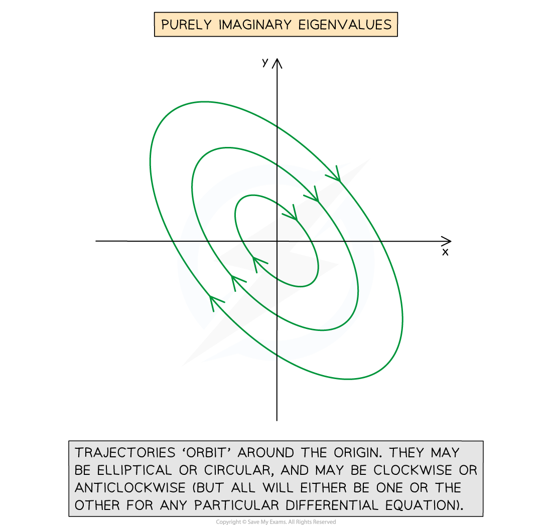
Real part is not equal to zero
Suppose
format('truetype')%3Bfont-weight%3Anormal%3Bfont-style%3Anormal%3B%7D%3C%2Fstyle%3E%3C%2Fdefs%3E%3Ctext%20font-family%3D%22Times%20New%20Roman%22%20font-size%3D%2218%22%20font-style%3D%22italic%22%20text-anchor%3D%22middle%22%20x%3D%224.5%22%20y%3D%2216%22%3E%26%23x3BB%3B%3C%2Ftext%3E%3Ctext%20font-family%3D%22Times%20New%20Roman%22%20font-size%3D%2213%22%20text-anchor%3D%22middle%22%20x%3D%2213.5%22%20y%3D%2224%22%3E1%3C%2Ftext%3E%3Ctext%20font-family%3D%22math1564b4c0e54101ac57a0cb68c16%22%20font-size%3D%2216%22%20text-anchor%3D%22middle%22%20x%3D%2225.5%22%20y%3D%2216%22%3E%3D%3C%2Ftext%3E%3Ctext%20font-family%3D%22Times%20New%20Roman%22%20font-size%3D%2218%22%20font-style%3D%22italic%22%20text-anchor%3D%22middle%22%20x%3D%2238.5%22%20y%3D%2216%22%3Ea%3C%2Ftext%3E%3Ctext%20font-family%3D%22math1564b4c0e54101ac57a0cb68c16%22%20font-size%3D%2216%22%20text-anchor%3D%22middle%22%20x%3D%2251.5%22%20y%3D%2216%22%3E%2B%3C%2Ftext%3E%3Ctext%20font-family%3D%22Times%20New%20Roman%22%20font-size%3D%2218%22%20font-style%3D%22italic%22%20text-anchor%3D%22middle%22%20x%3D%2264.5%22%20y%3D%2216%22%3Eb%3C%2Ftext%3E%3Ctext%20font-family%3D%22Times%20New%20Roman%22%20font-size%3D%2218%22%20text-anchor%3D%22middle%22%20x%3D%2272.5%22%20y%3D%2216%22%3Ei%3C%2Ftext%3E%3C%2Fsvg%3E) and
and format('truetype')%3Bfont-weight%3Anormal%3Bfont-style%3Anormal%3B%7D%3C%2Fstyle%3E%3C%2Fdefs%3E%3Ctext%20font-family%3D%22Times%20New%20Roman%22%20font-size%3D%2218%22%20font-style%3D%22italic%22%20text-anchor%3D%22middle%22%20x%3D%224.5%22%20y%3D%2216%22%3E%26%23x3BB%3B%3C%2Ftext%3E%3Ctext%20font-family%3D%22Times%20New%20Roman%22%20font-size%3D%2213%22%20text-anchor%3D%22middle%22%20x%3D%2213.5%22%20y%3D%2224%22%3E2%3C%2Ftext%3E%3Ctext%20font-family%3D%22math143f4d31b04031e49f5eb18baba%22%20font-size%3D%2216%22%20text-anchor%3D%22middle%22%20x%3D%2225.5%22%20y%3D%2216%22%3E%3D%3C%2Ftext%3E%3Ctext%20font-family%3D%22Times%20New%20Roman%22%20font-size%3D%2218%22%20font-style%3D%22italic%22%20text-anchor%3D%22middle%22%20x%3D%2238.5%22%20y%3D%2216%22%3Ea%3C%2Ftext%3E%3Ctext%20font-family%3D%22math143f4d31b04031e49f5eb18baba%22%20font-size%3D%2216%22%20text-anchor%3D%22middle%22%20x%3D%2251.5%22%20y%3D%2216%22%3E%26%23x2212%3B%3C%2Ftext%3E%3Ctext%20font-family%3D%22Times%20New%20Roman%22%20font-size%3D%2218%22%20font-style%3D%22italic%22%20text-anchor%3D%22middle%22%20x%3D%2264.5%22%20y%3D%2216%22%3Eb%3C%2Ftext%3E%3Ctext%20font-family%3D%22Times%20New%20Roman%22%20font-size%3D%2218%22%20text-anchor%3D%22middle%22%20x%3D%2272.5%22%20y%3D%2216%22%3Ei%3C%2Ftext%3E%3C%2Fsvg%3E)
To draw a solution trajectory
Find the direction at
or to determine if it is clockwise or counter-counterDraw spirals from origin
Label the direction of the trajectories
If
format('truetype')%3Bfont-weight%3Anormal%3Bfont-style%3Anormal%3B%7D%3C%2Fstyle%3E%3C%2Fdefs%3E%3Ctext%20font-family%3D%22Times%20New%20Roman%22%20font-size%3D%2218%22%20font-style%3D%22italic%22%20text-anchor%3D%22middle%22%20x%3D%224.5%22%20y%3D%2216%22%3Ea%3C%2Ftext%3E%3Ctext%20font-family%3D%22math1072b030ba126b2f4b2374f342b%22%20font-size%3D%2216%22%20text-anchor%3D%22middle%22%20x%3D%2217.5%22%20y%3D%2216%22%3E%26lt%3B%3C%2Ftext%3E%3Ctext%20font-family%3D%22Times%20New%20Roman%22%20font-size%3D%2218%22%20text-anchor%3D%22middle%22%20x%3D%2229.5%22%20y%3D%2216%22%3E0%3C%2Ftext%3E%3C%2Fsvg%3E) it spirals towards the origin
it spirals towards the originIf
format('truetype')%3Bfont-weight%3Anormal%3Bfont-style%3Anormal%3B%7D%3C%2Fstyle%3E%3C%2Fdefs%3E%3Ctext%20font-family%3D%22Times%20New%20Roman%22%20font-size%3D%2218%22%20font-style%3D%22italic%22%20text-anchor%3D%22middle%22%20x%3D%224.5%22%20y%3D%2216%22%3Ea%3C%2Ftext%3E%3Ctext%20font-family%3D%22math144f683a84163b3523afe57c2e0%22%20font-size%3D%2216%22%20text-anchor%3D%22middle%22%20x%3D%2217.5%22%20y%3D%2216%22%3E%26gt%3B%3C%2Ftext%3E%3Ctext%20font-family%3D%22Times%20New%20Roman%22%20font-size%3D%2218%22%20text-anchor%3D%22middle%22%20x%3D%2229.5%22%20y%3D%2216%22%3E0%3C%2Ftext%3E%3C%2Fsvg%3E) it spirals away from the origin
it spirals away from the origin
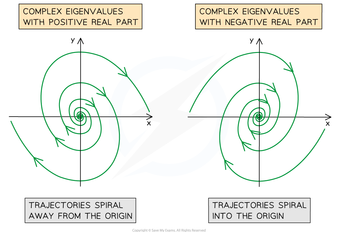
Worked Example
Consider the system of coupled differential equations
format('truetype')%3Bfont-weight%3Anormal%3Bfont-style%3Anormal%3B%7D%3C%2Fstyle%3E%3C%2Fdefs%3E%3Cline%20stroke%3D%22%23000%22%20stroke-linecap%3D%22square%22%20stroke-width%3D%221%22%20x1%3D%222.5%22%20x2%3D%2225.5%22%20y1%3D%2223.5%22%20y2%3D%2223.5%22%2F%3E%3Ctext%20font-family%3D%22Times%20New%20Roman%22%20font-size%3D%2218%22%20text-anchor%3D%22middle%22%20x%3D%229.5%22%20y%3D%2216%22%3Ed%3C%2Ftext%3E%3Ctext%20font-family%3D%22Times%20New%20Roman%22%20font-size%3D%2218%22%20font-style%3D%22italic%22%20text-anchor%3D%22middle%22%20x%3D%2218.5%22%20y%3D%2216%22%3Ex%3C%2Ftext%3E%3Ctext%20font-family%3D%22Times%20New%20Roman%22%20font-size%3D%2218%22%20text-anchor%3D%22middle%22%20x%3D%2211.5%22%20y%3D%2241%22%3Ed%3C%2Ftext%3E%3Ctext%20font-family%3D%22Times%20New%20Roman%22%20font-size%3D%2218%22%20font-style%3D%22italic%22%20text-anchor%3D%22middle%22%20x%3D%2218.5%22%20y%3D%2241%22%3Et%3C%2Ftext%3E%3Ctext%20font-family%3D%22math190bc3972c7934354efb2af01e7%22%20font-size%3D%2216%22%20text-anchor%3D%22middle%22%20x%3D%2236.5%22%20y%3D%2230%22%3E%3D%3C%2Ftext%3E%3Ctext%20font-family%3D%22math190bc3972c7934354efb2af01e7%22%20font-size%3D%2216%22%20text-anchor%3D%22middle%22%20x%3D%2253.5%22%20y%3D%2230%22%3E%26%23x2212%3B%3C%2Ftext%3E%3Ctext%20font-family%3D%22Times%20New%20Roman%22%20font-size%3D%2218%22%20text-anchor%3D%22middle%22%20x%3D%2266.5%22%20y%3D%2230%22%3E2%3C%2Ftext%3E%3Ctext%20font-family%3D%22Times%20New%20Roman%22%20font-size%3D%2218%22%20font-style%3D%22italic%22%20text-anchor%3D%22middle%22%20x%3D%2275.5%22%20y%3D%2230%22%3Ex%3C%2Ftext%3E%3Ctext%20font-family%3D%22math190bc3972c7934354efb2af01e7%22%20font-size%3D%2216%22%20text-anchor%3D%22middle%22%20x%3D%2289.5%22%20y%3D%2230%22%3E%2B%3C%2Ftext%3E%3Ctext%20font-family%3D%22Times%20New%20Roman%22%20font-size%3D%2218%22%20text-anchor%3D%22middle%22%20x%3D%22102.5%22%20y%3D%2230%22%3E2%3C%2Ftext%3E%3Ctext%20font-family%3D%22Times%20New%20Roman%22%20font-size%3D%2218%22%20font-style%3D%22italic%22%20text-anchor%3D%22middle%22%20x%3D%22111.5%22%20y%3D%2230%22%3Ey%3C%2Ftext%3E%3Cline%20stroke%3D%22%23000%22%20stroke-linecap%3D%22square%22%20stroke-width%3D%221%22%20x1%3D%222.5%22%20x2%3D%2225.5%22%20y1%3D%2274.5%22%20y2%3D%2274.5%22%2F%3E%3Ctext%20font-family%3D%22Times%20New%20Roman%22%20font-size%3D%2218%22%20text-anchor%3D%22middle%22%20x%3D%229.5%22%20y%3D%2267%22%3Ed%3C%2Ftext%3E%3Ctext%20font-family%3D%22Times%20New%20Roman%22%20font-size%3D%2218%22%20font-style%3D%22italic%22%20text-anchor%3D%22middle%22%20x%3D%2218.5%22%20y%3D%2267%22%3Ey%3C%2Ftext%3E%3Ctext%20font-family%3D%22Times%20New%20Roman%22%20font-size%3D%2218%22%20text-anchor%3D%22middle%22%20x%3D%2211.5%22%20y%3D%2292%22%3Ed%3C%2Ftext%3E%3Ctext%20font-family%3D%22Times%20New%20Roman%22%20font-size%3D%2218%22%20font-style%3D%22italic%22%20text-anchor%3D%22middle%22%20x%3D%2218.5%22%20y%3D%2292%22%3Et%3C%2Ftext%3E%3Ctext%20font-family%3D%22math190bc3972c7934354efb2af01e7%22%20font-size%3D%2216%22%20text-anchor%3D%22middle%22%20x%3D%2236.5%22%20y%3D%2281%22%3E%3D%3C%2Ftext%3E%3Ctext%20font-family%3D%22Times%20New%20Roman%22%20font-size%3D%2218%22%20font-style%3D%22italic%22%20text-anchor%3D%22middle%22%20x%3D%2249.5%22%20y%3D%2281%22%3Ex%3C%2Ftext%3E%3Ctext%20font-family%3D%22math190bc3972c7934354efb2af01e7%22%20font-size%3D%2216%22%20text-anchor%3D%22middle%22%20x%3D%2263.5%22%20y%3D%2281%22%3E%26%23x2212%3B%3C%2Ftext%3E%3Ctext%20font-family%3D%22Times%20New%20Roman%22%20font-size%3D%2218%22%20text-anchor%3D%22middle%22%20x%3D%2276.5%22%20y%3D%2281%22%3E3%3C%2Ftext%3E%3Ctext%20font-family%3D%22Times%20New%20Roman%22%20font-size%3D%2218%22%20font-style%3D%22italic%22%20text-anchor%3D%22middle%22%20x%3D%2285.5%22%20y%3D%2281%22%3Ey%3C%2Ftext%3E%3C%2Fsvg%3E)
Given that ![]() and
and ![]() are the eigenvalues of the matrix
are the eigenvalues of the matrix format('truetype')%3Bfont-weight%3Anormal%3Bfont-style%3Anormal%3B%7D%40font-face%7Bfont-family%3A'brack_sm2882ad605b1e27be87c7468'%3Bsrc%3Aurl(data%3Afont%2Ftruetype%3Bcharset%3Dutf-8%3Bbase64%2CAAEAAAAMAIAAAwBAT1MvMi7PH4UAAADMAAAATmNtYXA3kjw6AAABHAAAADxjdnQgAQYDiAAAAVgAAAASZ2x5ZkyYQ7YAAAFsAAAAkWhlYWQLyR8fAAACAAAAADZoaGVhAq0XCAAAAjgAAAAkaG10eDEjA%2FUAAAJcAAAADGxvY2EAAEKZAAACaAAAABBtYXhwBJsEcQAAAngAAAAgbmFtZW7QvZAAAAKYAAAB5XBvc3QArQBVAAAEgAAAACBwcmVwu5WEAAAABKAAAAAHAAACDAGQAAUAAAQABAAAAAAABAAEAAAAAAAAAQEAAAAAAAAAAAAAAAAAAAAAAAAAAAAAAAAAAAAAACAgICAAAAAg9AMD%2FP%2F8AAABVAABAAAAAAACAAEAAQAAABQAAwABAAAAFAAEACgAAAAGAAQAAQACI5wjn%2F%2F%2FAAAjnCOf%2F%2F%2FcZdxjAAEAAAAAAAAAAAFUAFQBAAArAIwAgACoAAcAAAACAAAAAADVAQEAAwAHAAAxMxEjFyM1M9XVq4CAAQHWqwABAAAAAABVAVgAAwAfGAGwAy%2BwADyxAgL1sAE8ALEDAD%2BwAjx8sQAG9bABPBEzESNVVQFY%2FqgAAQDXAAABLAFUAAMAIBgBsAUvsAE8sAI8sQAC9bADPACwAy%2BwAjyxAAH1sAE8EzMRI9dVVQFU%2FqwAAAAAAQAAAAEAAIsesexfDzz1AAMEAP%2F%2F%2F%2F%2FVre5k%2F%2F%2F%2F%2F9Wt7mT%2FgP%2F%2FAdYBWAAAAAoAAgABAAAAAAABAAABVP%2F%2FAAAXcP%2BA%2F4AB1gABAAAAAAAAAAAAAAAAAAAAAwDVAAABLAAAASwA1wAAAAAAAAAhAAAAWAAAAJEAAQAAAAMACgACAAAAAAACAIAEAAAAAAAEAABlAAAAAAAAABUBAgAAAAAAAAABACYAAAAAAAAAAAACAA4AJgAAAAAAAAADAEQANAAAAAAAAAAEACYAeAAAAAAAAAAFABYAngAAAAAAAAAGABMAtAAAAAAAAAAIABwAxwABAAAAAAABACYAAAABAAAAAAACAA4AJgABAAAAAAADAEQANAABAAAAAAAEACYAeAABAAAAAAAFABYAngABAAAAAAAGABMAtAABAAAAAAAIABwAxwADAAEECQABACYAAAADAAEECQACAA4AJgADAAEECQADAEQANAADAAEECQAEACYAeAADAAEECQAFABYAngADAAEECQAGABMAtAADAAEECQAIABwAxwBCAHIAYQBjAGsAZQB0AHMAIABzAG0AYQBsAGwAIABzAGkAegBlAFIAZQBnAHUAbABhAHIATQBhAHQAaABzACAARgBvAHIAIABNAG8AcgBlACAAQgByAGEAYwBrAGUAdABzACAAcwBtAGEAbABsACAAcwBpAHoAZQBCAHIAYQBjAGsAZQB0AHMAIABzAG0AYQBsAGwAIABzAGkAegBlAFYAZQByAHMAaQBvAG4AIAAyAC4AMEJyYWNrZXRzX3NtYWxsX3NpemUATQBhAHQAaABzACAARgBvAHIAIABNAG8AcgBlAAAAAAMAAAAAAAAAqgBVAAAAAAAAAAAAAAAAAAAAAAAAAAC5B%2F8AAo2FAA%3D%3D)format('truetype')%3Bfont-weight%3Anormal%3Bfont-style%3Anormal%3B%7D%40font-face%7Bfont-family%3A'bracketse552f5417ff4680c6b50499'%3Bsrc%3Aurl(data%3Afont%2Ftruetype%3Bcharset%3Dutf-8%3Bbase64%2CAAEAAAAMAIAAAwBAT1MvMi7RIisAAADMAAAATmNtYXBi7uzYAAABHAAAAExjdnQgBAkDLgAAAWgAAAASZ2x5Zo64f%2BkAAAF8AAABSWhlYWQLniGcAAACyAAAADZoaGVhBK4XLAAAAwAAAAAkaG10eCWq%2F90AAAMkAAAAFGxvY2EAABknAAADOAAAABhtYXhwBJIESAAAA1AAAAAgbmFtZRAA8I4AAANwAAAB3nBvc3QBwwDgAAAFUAAAACBwcmVwupWEAAAABXAAAAAHAAACggGQAAUAAAQABAAAAAAABAAEAAAAAAAAAQEAAAAAAAAAAAAAAAAAAAAAAAAAAAAAAAAAAAAAACAgICAAAAAg9AMEAAAAAAADgAAAAAAAAAACAAEAAQAAABQAAwABAAAAFAAEADgAAAAKAAgAAgACI5sjnSOeI6D%2F%2FwAAI5sjnSOeI6D%2F%2F9xm3GXcZdxkAAEAAAAAAAAAAAAAAAABVABWAQAALACoA4AAMgAHAAAAAgAAACoA1QNVAAMABwAANTMRIxMjETPV1auAgCoDK%2F0AAtUAAQAAAAABgAOAAAUAJBgBsAAvsAPFsQEC%2FbADELEEBP0AsQAAP7ABPLEEBj%2BwAzwwMTEzEAEjAFUBKyv%2BqwH8AYT%2BqgABAAAAAAGAA4AABQAmGAGwAC6wA8WxBQL9sAMQsQIE%2FQB8sQAGPxiwBTyxAwb2sAI8MDEREgEzABMBAVQr%2FtMCA4D91v6qAYQB%2FAAB%2F6wAAAEsA4AABQAnGAGwAC%2BwBzywA8WxAQL9sAMQsQQE%2FQCxAAA%2FsAE8sQQGP7ADPDAxISMSATMAASxVAf7UKwFVAfwBhP6rAAH%2FrAAAASwDgAAFACkYAbABL7AHPLAExbEAAv2wBBCxAwT9AHyxAQY%2FsAA8GLEEAD%2BwAzwwMRMzEAEjANdV%2FqsrASsDgP3V%2FqsBhgAAAAABAAAAAQAAeuTcpl8PPPUAAwQA%2F%2F%2F%2F%2F9Wt7o7%2F%2F%2F%2F%2F1a3ujv%2BsAAABgAOAAAAACgACAAEAAAAAAAEAAAOAAAAAABdw%2F6z%2FrAGAAAEAAAAAAAAAAAAAAAAAAAAFANUAAAEsAAABLAAAASz%2FrAEs%2F6wAAAAAAAAAJAAAAGgAAACzAAAA%2FQAAAUkAAQAAAAUACAACAAAAAAACAIAEAAAAAAAEAAA%2BAAAAAAAAABUBAgAAAAAAAAABACQAAAAAAAAAAAACAA4AJAAAAAAAAAADAEIAMgAAAAAAAAAEACQAdAAAAAAAAAAFABYAmAAAAAAAAAAGABIArgAAAAAAAAAIABwAwAABAAAAAAABACQAAAABAAAAAAACAA4AJAABAAAAAAADAEIAMgABAAAAAAAEACQAdAABAAAAAAAFABYAmAABAAAAAAAGABIArgABAAAAAAAIABwAwAADAAEECQABACQAAAADAAEECQACAA4AJAADAAEECQADAEIAMgADAAEECQAEACQAdAADAAEECQAFABYAmAADAAEECQAGABIArgADAAEECQAIABwAwABCAHIAYQBjAGsAZQB0AHMAIABmAHUAbABsACAAcwBpAHoAZQBSAGUAZwB1AGwAYQByAE0AYQB0AGgAcwAgAEYAbwByACAATQBvAHIAZQAgAEIAcgBhAGMAawBlAHQAcwAgAGYAdQBsAGwAIABzAGkAegBlAEIAcgBhAGMAawBlAHQAcwAgAGYAdQBsAGwAIABzAGkAegBlAFYAZQByAHMAaQBvAG4AIAAyAC4AMEJyYWNrZXRzX2Z1bGxfc2l6ZQBNAGEAdABoAHMAIABGAG8AcgAgAE0AbwByAGUAAAADAAAAAAAAAcAA4AAAAAAAAAAAAAAAAAAAAAAAAAAAuQf%2FAAGNhQA%3D)format('truetype')%3Bfont-weight%3Anormal%3Bfont-style%3Anormal%3B%7D%3C%2Fstyle%3E%3C%2Fdefs%3E%3Ctext%20font-family%3D%22bracketse552f5417ff4680c6b50499%22%20font-size%3D%2218%22%20text-anchor%3D%22start%22%20x%3D%221.5%22%20y%3D%2218%22%3E%26%23x239B%3B%3C%2Ftext%3E%3Ctext%20font-family%3D%22brack_sm2882ad605b1e27be87c7468%22%20font-size%3D%2218%22%20text-anchor%3D%22start%22%20x%3D%221.5%22%20y%3D%2224%22%3E%26%23x239C%3B%3C%2Ftext%3E%3Ctext%20font-family%3D%22brack_sm2882ad605b1e27be87c7468%22%20font-size%3D%2218%22%20text-anchor%3D%22start%22%20x%3D%221.5%22%20y%3D%2230%22%3E%26%23x239C%3B%3C%2Ftext%3E%3Ctext%20font-family%3D%22brack_sm2882ad605b1e27be87c7468%22%20font-size%3D%2218%22%20text-anchor%3D%22start%22%20x%3D%221.5%22%20y%3D%2236%22%3E%26%23x239C%3B%3C%2Ftext%3E%3Ctext%20font-family%3D%22bracketse552f5417ff4680c6b50499%22%20font-size%3D%2218%22%20text-anchor%3D%22start%22%20x%3D%221.5%22%20y%3D%2252%22%3E%26%23x239D%3B%3C%2Ftext%3E%3Ctext%20font-family%3D%22bracketse552f5417ff4680c6b50499%22%20font-size%3D%2218%22%20text-anchor%3D%22start%22%20x%3D%2268.5%22%20y%3D%2218%22%3E%26%23x239E%3B%3C%2Ftext%3E%3Ctext%20font-family%3D%22brack_sm2882ad605b1e27be87c7468%22%20font-size%3D%2218%22%20text-anchor%3D%22start%22%20x%3D%2268.5%22%20y%3D%2224%22%3E%26%23x239F%3B%3C%2Ftext%3E%3Ctext%20font-family%3D%22brack_sm2882ad605b1e27be87c7468%22%20font-size%3D%2218%22%20text-anchor%3D%22start%22%20x%3D%2268.5%22%20y%3D%2230%22%3E%26%23x239F%3B%3C%2Ftext%3E%3Ctext%20font-family%3D%22brack_sm2882ad605b1e27be87c7468%22%20font-size%3D%2218%22%20text-anchor%3D%22start%22%20x%3D%2268.5%22%20y%3D%2236%22%3E%26%23x239F%3B%3C%2Ftext%3E%3Ctext%20font-family%3D%22bracketse552f5417ff4680c6b50499%22%20font-size%3D%2218%22%20text-anchor%3D%22start%22%20x%3D%2268.5%22%20y%3D%2252%22%3E%26%23x23A0%3B%3C%2Ftext%3E%3Ctext%20font-family%3D%22math1da40657c9fece7e48d30af42d3%22%20font-size%3D%2216%22%20text-anchor%3D%22middle%22%20x%3D%2217.5%22%20y%3D%2219%22%3E%26%23x2212%3B%3C%2Ftext%3E%3Ctext%20font-family%3D%22Times%20New%20Roman%22%20font-size%3D%2218%22%20text-anchor%3D%22middle%22%20x%3D%2228.5%22%20y%3D%2219%22%3E2%3C%2Ftext%3E%3Ctext%20font-family%3D%22Times%20New%20Roman%22%20font-size%3D%2218%22%20text-anchor%3D%22middle%22%20x%3D%2251.5%22%20y%3D%2219%22%3E2%3C%2Ftext%3E%3Ctext%20font-family%3D%22Times%20New%20Roman%22%20font-size%3D%2218%22%20text-anchor%3D%22middle%22%20x%3D%2221.5%22%20y%3D%2245%22%3E1%3C%2Ftext%3E%3Ctext%20font-family%3D%22math1da40657c9fece7e48d30af42d3%22%20font-size%3D%2216%22%20text-anchor%3D%22middle%22%20x%3D%2247.5%22%20y%3D%2245%22%3E%26%23x2212%3B%3C%2Ftext%3E%3Ctext%20font-family%3D%22Times%20New%20Roman%22%20font-size%3D%2218%22%20text-anchor%3D%22middle%22%20x%3D%2258.5%22%20y%3D%2245%22%3E3%3C%2Ftext%3E%3C%2Fsvg%3E) , with corresponding eigenvectors
, with corresponding eigenvectors ![]() and
and ![]() , draw a phase portrait for the solutions of the system.
, draw a phase portrait for the solutions of the system.
Answer:


Unlock more, it's free!
Join the 100,000+ Students that ❤️ Save My Exams
the (exam) results speak for themselves:

Was this revision note helpful?