Practical Skills & Data Analysis (Paper 3A) (AQA A Level Physics): Exam Questions

Figure 1 is a plot of current–voltage data for a filament lamp L.

Figure 1

The current $I$ was measured as the voltage $V$ across L was increased at a steady rate.

These data were obtained using a current sensor and a voltage sensor connected to a data logger.

The logger recorded data at a rate of $2.5\mathrm{Hz}$.

Determine, in $\mathrm{V}{\mathrm{s}}^{-1}$ , the rate of increase of $V$.

State two advantages of using data logging for this experiment.

Figure 2 shows two circuits that can be used to collect current–voltage data.

Figure 2

The dc supply has an emf of $12\mathrm{V}$ and negligible internal resistance.

The current sensor and the voltage sensor behave as ideal meters.

In circuit 1:

• X is used as a variable resistor with a maximum resistance of $14.9\mathrm{\Omega }$

• when X is set to maximum resistance, the resistance of L is $2.3\mathrm{\Omega }$.

In circuit 2, X is used as a potential divider.

Discuss, with reference to circuit 1 and circuit 2, whether either circuit can produce all the data shown in Figure 1.
Support your answer with a calculation.

Table 1 shows some values of $V$ that are plotted on Figure 1 and corresponding results for $I$ and for the power $P$ dissipated in L.

Table 1

Complete Table 1.

Plot on Figure 3 a graph of $P$ against $V$. You should use only the data in your completed Table 1.

Figure 6

L is connected to a $12\mathrm{V}$ power supply of negligible internal resistance.

L then dissipates its rated power $P_r$ .

A second lamp, identical to L, is now connected in series with L.

Determine the percentage of $P_r$ that is dissipated in this circuit.

This question is based on the ideas behind required practical activity 11 - investigating the effect on magnetic flux linkage using a search coil.

Figure 1 shows the front view of a vertical coil mounted on a circular frame.

Figure 1 also includes a side view showing a section through the frame and coil.
A constant direct current in the coil produces magnetic flux represented by the magnetic field lines on this diagram.

Figure 1

Point Q is at the centre of the coil.
A sensor placed at Q detects $B_H$, the horizontal component of the magnetic flux density.
The effect of the Earth’s magnetic field at Q is negligible.

Discuss whether a search coil is a suitable sensor to detect $B_H$.

$B_H$ is measured at Q with the coil vertical.

The coil is now rotated about Q through $25°$ as shown in Figure 2.
The current in the coil does not change.

Figure 2

A new measurement of $B_H$ is made with the coil fixed in this new position.

Determine the percentage change in $B_H$ produced by this rotation of the coil.
Show your working.

Figure 3 shows a protractor being used to measure the angle through which the coil is rotated.

Figure 3

Estimate the percentage uncertainty in this result.
Justify your answer.

Figure 4 shows an arrangement of two vertical coils.
Four experiments are done using this arrangement.

Figure 4

Coil 1 and coil 2 are identical and have a radius $r$.
The coils are separated by a distance $r$ and have a common axis PR.
Q is at the centre of coil 1.

The four different experiments investigate how $B_H$ varies with $x$, the displacement of the sensor from Q along PR.

In experiment 1, the current in coil 1 is $225\mathrm{mA}$and the current in coil 2 is zero.

In experiment 2, the current in coil 1 is zero and the current in coil 2 is $225\mathrm{mA}$.

Figure 5 shows the results of experiment 1 and experiment 2.

Figure 5

During experiment 1, $B_H$ is measured with the sensor at Q.
The sensor is then moved along PR until the value of $B_H$ is halved.
The distance from Q to the sensor is $x_{0.5}$.

Determine $\frac{x_{0.5}}{r}$

In experiment 3, the current in both coils is $225\mathrm{mA}$ so that the magnetic fields produced by coil 1 and coil 2 are combined.

The resultant $B_H$ has a constant maximum value in the region between $x=\frac{r}{4}$ and $x=\frac{3r}{4}$

Deduce, in $\mathrm{mT}$, the value of $B_H$ in this region.

State two characteristics of the magnetic field lines in this region.

In experiment 4, the current in coil 2 is reversed so that the direction of the magnetic field produced by coil 2 is also reversed.
The magnitudes of the currents in coil 1 and coil 2 are still $225\mathrm{mA}$.

Sketch a graph to show how $B_H$ varies between $x=0$ and $x=r$.
The $x$-axis has been provided for you.

Your graph should include numerical values on your $B_H$ axis that correspond to $x=0$ and $x=r$.

This question is based on a method to investigate Boyle's law (required practical activity 8).

Figure 1 shows air trapped in a vertical cylinder by a valve and a piston P.
The valve remains closed throughout the experiment.

A mass is placed on top of P.
P moves downwards and the volume of the trapped air decreases.
There are no air leaks and there is no friction between the cylinder and P.

Figure 1

The vertical distance $y$ between the end of P and the closed end of the cylinder is measured.
Additional masses are used to find out how $y$ depends on the total mass $M$ placed on top of P.
Figure 2 shows a graph of these data.

Show that $y$ is not inversely proportional to $M$.
Use data points from Figure 2.

Figure 2

The masses are removed, and the cylinder is inverted.

P moves downwards without friction before coming to rest, as shown in Figure 3.

Figure 3

Explain why P does not fall out of the cylinder unless the valve is opened.

The mass of P is $0.350\mathrm{kg}$.

Deduce $y$ when the cylinder is in the inverted position shown in Figure 3.

Draw a line of best fit on Figure 2 to arrive at your answer.

Figure 4 shows apparatus used in schools to investigate Boyle’s law.

Figure 4

A fixed mass of air is trapped above some coloured oil inside a glass tube, closed at the top.
A pump applies pressure to the oil and the air.
The trapped air is compressed and its pressure $p$ is read from the pressure gauge.

A scale, marked in $0.2{\mathrm{cm}}^3$ intervals, is used to measure the volume $V$ of the air.
A student says that the reading for $V$ shown in Figure 4 is $35.4{\mathrm{cm}}^3$.

State:

• the error the student has made

• the correct reading, in ${\mathrm{cm}}^3$, of the volume.

Figure 5 shows data obtained using the apparatus in Figure 4.

Figure 5

Explain why the gradient of the graph in Figure 5 confirms that the air obeys Boyle’s law.

The largest pressure that can be read from the pressure gauge is $3.4\times {10}^5\mathrm{Pa}$.

Determine, using Figure 5, the volume $V$ corresponding to this pressure.

State one property of the air that must not change during the experiment.
Go on to suggest how this can be achieved.

This question is based on required practical activity 2 - investigating interference using a diffraction grating.

A light-emitting diode (LED) emits light over a narrow range of wavelengths.
These wavelengths are distributed about a peak wavelength ${\lambda }_p$.

Two LEDs L_G and L_R are adjusted to give the same maximum light intensity.
L_G emits green light and L_R emits red light.

Figure 1 shows how the light output of the LEDs varies with the wavelength $\lambda$.

Figure 1

Light from L_R is incident normally on a plane diffraction grating.
The fifth-order maximum for light of wavelength ${\lambda }_p$ occurs at a diffraction angle of $76.3°$.

Determine $N$, the number of lines per metre on the grating.

Suggest one possible disadvantage of using the fifth-order maximum to determine $N$.

Figure 2 shows part of the current−voltage characteristics for L_R and L_G.

Figure 2

When the linear part of the characteristic is extrapolated, the point at which it meets the horizontal axis gives the activation voltage $V_A$ for the LED.

$V_A$ for L_G is $2.00\mathrm{V}$.

Determine, using Figure 2, $V_A$ for L_R.

It can be shown that:

$V_A=\frac{hc}{e{\lambda }_p}$

where $h$ = the Planck constant.

Deduce a value for the Planck constant based on the data given about the LEDs.

Figure 3 shows a circuit with L_R connected to a resistor of resistance $R$.

Figure 3

The power supply has emf $6.10\mathrm{V}$ and negligible internal resistance.

The current in L_R must not exceed $21.0\mathrm{mA}$.

Deduce the minimum value of $R$.

This question is based on Required Practical 9: Investigation of the charge and discharge of capacitors.

An analogue voltmeter has a resistance that is much less than that of a modern digital voltmeter.
Analogue meters can be damaged if the full-scale reading is exceeded.
Figure 1 shows a dual-range analogue voltmeter with a zero error.

Figure 1

The voltmeter is set to the more sensitive range and then used in a circuit.

What is the potential difference (pd) between the terminals of the voltmeter when a full-scale reading is indicated?

Explain the use of the mirror when reading the meter.

A student corrects the zero error on the meter and then assembles the circuit shown in Figure 2.
The capacitance of the capacitor C is not known.

Figure 2

The output pd of the power supply is set to zero.
The student connects the flying lead to socket X and adjusts the output pd until the voltmeter reading is full scale $\left(15\mathrm{V}\right)$.
She disconnects the flying lead from socket X so that C discharges through the voltmeter.

She measures the time $T_{1/2}$ for the voltmeter reading $V$ to fall from $10\mathrm{V}$ to $5\mathrm{V}$.
She repeats this process several times.

Table 1 shows the student’s results, none of which is anomalous.

Table 1

Determine the percentage uncertainty in $T_{1/2}$.

Show that the time constant for the discharge circuit is about $17\mathrm{s}$.

The student thinks that the time constant of the circuit in Figure 2 is directly proportional to the range of the meter.
To test her theory, she repeats the experiment with the voltmeter set to the $3\mathrm{V}$ range.
She expects $T_{1/2}$ to be about $2.5\mathrm{s}$.

Explain:

• what the student should do, before connecting capacitor C to the $0\mathrm{V}$ and $3\mathrm{V}$ sockets, to avoid exceeding the full-scale reading on the voltmeter

• how she should develop her procedure to get an accurate result for the time constant

• how she should use her result to check whether her theory is correct.

The student wants to find the resistance of the voltmeter when it is set to the $15\mathrm{V}$ range.
She replaces C with an $820\mathrm{\mu F}$ capacitor and charges it to $15\mathrm{V}$.
She discharges the capacitor through the voltmeter, starting a stopwatch when $V$ is $14\mathrm{V}$.

She records the stopwatch reading $t$ at other values of $V$ as the capacitor discharges.

Table 2 shows her results.

Table 2

Suggest two reasons why the student selected the values of $V$ shown in Table 2.

Explain each of your answers.

Figure 3 shows a graph of the experimental data.

Figure 3

Show, using Figure 3, that the resistance of the voltmeter is about $16\mathrm{k\Omega }$.

Determine the current in the voltmeter at $t=10\mathrm{s}$.

This question is about required practical activity 6.

Figure 1 shows a partly-completed circuit used to investigate the emf $\epsilon$ and the internal resistance $r$ of a power supply.

The resistance of P and the maximum resistance of Q are unknown.

Figure 1

Complete Figure 1 to show a circuit including a voltmeter and an ammeter that is suitable for the investigation.

Describe

• a procedure to obtain valid experimental data using your circuit

• how these data are processed to obtain $\epsilon$ and $r$ by a graphical method.

Figure 2 shows a different experiment carried out to confirm the results for $\epsilon$ and $r$.

Figure 2

Initially the power supply is connected in series with an ammeter and a $22\mathrm{\Omega }$ resistor.
The current $I$ in the circuit is measured.

The number $n$ of $22\mathrm{\Omega }$ resistors in the circuit is increased as shown in Figure 2.
The current $I$ is measured after each resistor is added.

It can be shown that

$\frac{22}{n}=\frac{\epsilon }{I}-r$

Figure 3 shows a graph of the experimental data.

Figure 3

Show that $\epsilon$ is about $1.6\mathrm{V}$.

Figure 4 shows the circuit when four resistors are connected.

Figure 4

Show, using Figure 3, that the current in the power supply is about $0.25\mathrm{A}$.

Deduce, for the circuit shown in Figure 4,

• the potential difference (pd) across the power supply

• $r$.

Figure 5 shows the plots for $n=1$ and $n=14$

Figure 5

Three additional data sets for values of $n$ between $n=1$ and $n=14$ are needed to complete the graph in Figure 5.

Suggest which additional values of $n$ should be used.
Justify your answer.

The experiment is repeated using a set of resistors of resistance $27\mathrm{\Omega }$. The relationship between $n$ and $I$ is now

$\frac{27}{n}=\frac{\epsilon }{I}-r$

Show on Figure 5 the effect on the plots for $n=1$ and $n=14$
You do not need to do a calculation.

Figure 1 shows apparatus used to investigate the rate at which water flows through a horizontal cylindrical tube T of internal diameter $d$ and length $L$.

Figure 1

The apparatus ensures that the water level in the can is at a constant height $h$ above the centre of T.

Water flows out of T at a steady rate.

The volume flow rate through T is $Q$, where $Q$ is in ${\mathrm{mm}}^3{\mathrm{s}}^{-1}$.
A student wants to measure $Q$ as water flows through T.

Outline a procedure the student should follow to measure $Q$.
Include in your answer

• the measuring instruments used

• how uncertainty in the measurements can be reduced.

It can be shown that

$Q=\frac{\mathrm{\pi }\rho gh{d}^4}{128L\eta }$

where

• $\rho$ is the density of water

• $g$ is the gravitational field strength

• $\eta$ is a property of the water called the coefficient of viscosity.

What is the SI unit for $\eta$?

An experiment is carried out to determine $\eta$ by a graphical method.
The rate at which water flows out of T is varied by adjusting the height of the drain tube as shown in Figure 2.

Figure 2

During the experiment the temperature is kept constant.
$Q$ is found for different values of $h$ and a graph of these data is plotted, with $Q$ on the vertical axis.
The percentage uncertainty in the gradient of the graph is 6.4%.

The dimensions of tube T are measured and the uncertainties in these data are calculated.

The percentage uncertainty

• in $d$ is 2.9%

• in $L$ is 1.8%.

The percentage uncertainties in $\rho$and $g$ are negligible.

Deduce the percentage uncertainty in the result for $\eta$.

In a different experiment, the horizontal tube T is connected to a vertical glass tube.
Marks have been made at regular intervals on the glass tube.
The student measures and records the vertical distance $y$ between each of the marks and the centre of T.

She seals the open end of T and fills the glass tube with water, as shown in Figure 3.

Figure 3

T is opened and water flows into a beaker.
When the water level falls to the highest mark on the tube, she starts a stopwatch.
She records the time $t$ for the water to reach each of the other marks.

Explain how the student could check that the glass tube was vertical.
You may wish to add detail to Figure 3 to illustrate your answer.

Figure 4 shows part of the graph drawn from the student’s data.

Figure 4

It can be shown that $y$ decreases exponentially with $t$.

Show that $\lambda$, the decay constant for this process, is about $4.5\times {10}^{-3}{\mathrm{s}}^{-1}$.

$T_{1/2}$ is the time for $y$ to decrease by 50%, as shown in Figure 5.

Figure 5

Determine $T_{1/2}$.

The apparatus is adjusted so that the glass tube is inclined at 30° to the horizontal tube T, as shown in Figure 6.

Figure 6

The student measures and records the new values of $y$, the mean vertical distance between each of the marks and the centre of T.
She then carries out the experiment as before, recording new values of $t$ corresponding to each new value of $y$.

Draw a line on Figure 7 to show the graph produced using the modified apparatus.
The dashed line is the original graph when the glass tube was vertical as shown in Figure 3.

Figure 7

This question is about an experiment with a retractable steel tape measure.

The tape measure is placed at the edge of the bench and about $1\mathrm{m}$ of the steel tape is extended so that it overhangs the bench.

The tape is then locked in this position to stop it from retracting.

A student measures the dimensions $x$ and $y$, the horizontal and vertical displacements of the free end of the tape, as shown in Figure 1.

Figure 1

Describe a suitable procedure the student could use to measure $y$.
You may add detail to Figure 1 to illustrate your answer.

By changing the extension of the tape, the student obtains further values of $x$ and $y$.

These data are shown in Table 1.

Table 1

Suggest why the student chose to make all measurements of $x$ greater than $70\mathrm{cm}$.

The data from the experiment suggest that $y=A{x}^n$ where $n$ is an integer and $A$ is a constant.

These data are used to plot the graph in Figure 2.

Determine $n$ using Figure 2.

Figure 2

Explain how the numerical value of $A$ can be obtained from Figure 2.

Estimate the order of magnitude of $A$.
You should use data for $x$ and $y$ from any one row in Table 1.
Give your answer with an appropriate unit.

This question is about an investigation into how the first harmonic frequency of a stretched string varies with tension (required practical activity 1).

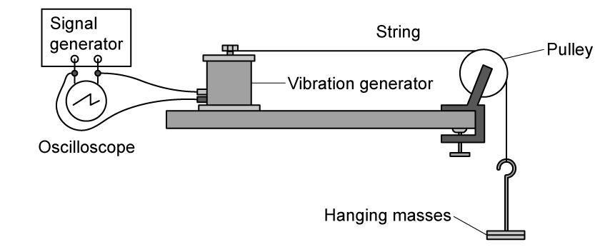
The apparatus used for this investigation is shown in Figure 1.

Figure 1

The tension $T$ in the string is varied by adding masses to a mass hanger suspended over a pulley.

For each mass, the frequency of the signal generator is adjusted until the string vibrates at its first harmonic frequency $f$.

State two variables that must be kept constant in this investigation.

Describe a suitable procedure a student could use to determine $f$.

You may add detail to Figure 1 to illustrate your answer.

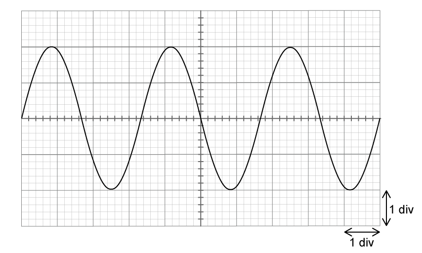
The oscilloscope is used to determine the frequency of the output of the signal generator.

Figure 2 shows the waveform displayed on the oscilloscope when $T=3.00\mathrm{N}$.

Figure 2

The time-base setting of the oscilloscope is $5.0\mathrm{ms}{\mathrm{div}}^{-1}$.

Determine $f$, the frequency of the waveform.

The student records the first harmonic frequency $f$ for five different values of tension, $T$.

The results are shown in Table 1.

Table 1

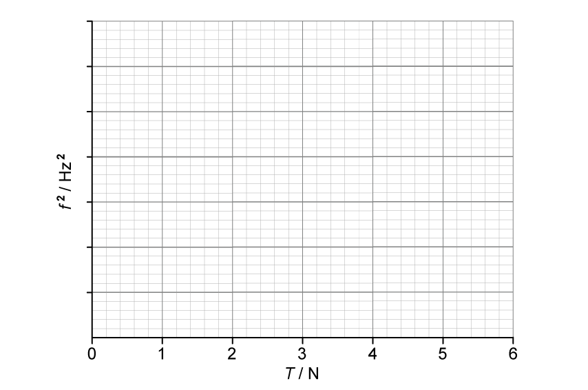
Plot on Figure 3 a graph of $f^2$ against $T$.

Record your values of $f^2$ in Table 1.

Figure 3

It can be shown that

$f=\frac{1}{2L}\sqrt{\frac{T}{\mu }}$

where $L=0.600\mathrm{m}$ and $\mu$ is the mass per unit length of the string.

Determine $\mu$ using Figure 3.

The student determines the value of $\mu$ to be $6.3\times {10}^{-4}{\text{ kg m}}^{-1}$.

Calculate the percentage difference between your value of $\mu$ from (e) and the student's value.

Suggest one reason for this difference related to the experimental procedure.

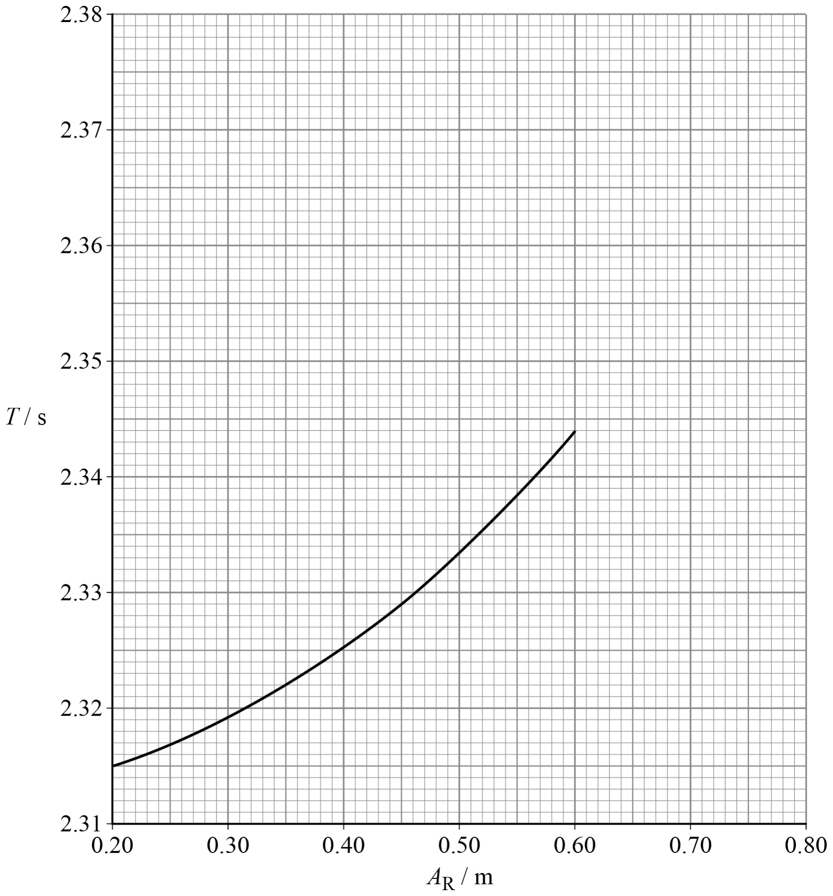
This question is about an investigation into the oscillation of a loaded metal strip.

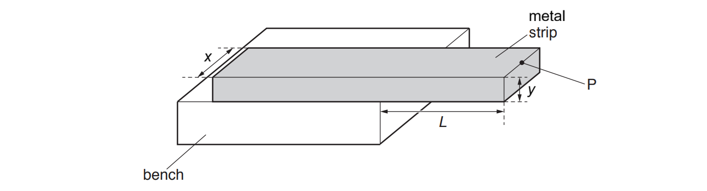
Figure 4 shows a rectangular metal strip of width $x$ and thickness $y$ clamped to a bench. A length $L$ of the strip extends horizontally over the edge of the bench.

Figure 4

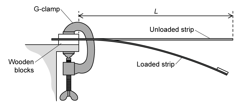
A load of mass $M$ is attached to the free end of the strip at P. This causes the unsupported part of the strip to bend, as shown in Figure 5.

Figure 5

The mass is displaced vertically and released so that it undergoes vertical oscillations of small amplitude. The period of the oscillations is $T$.

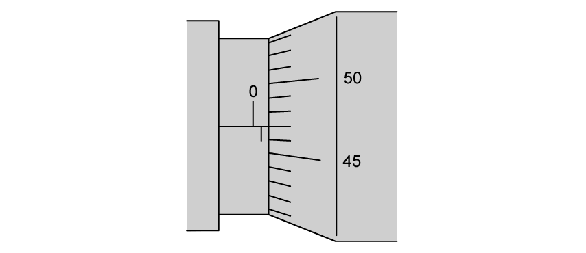
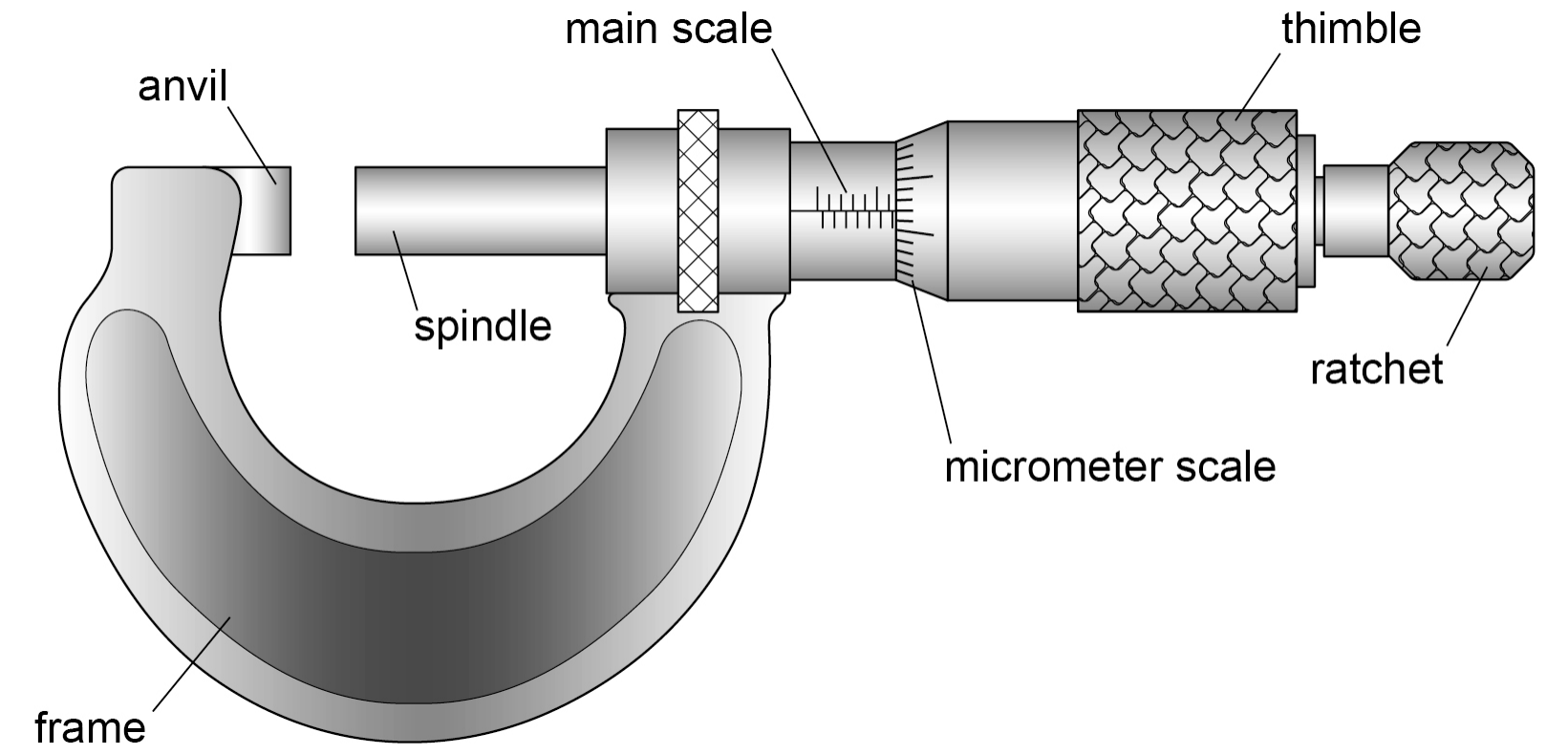
The student uses a micrometer to measure the thickness $y$ of the metal strip.

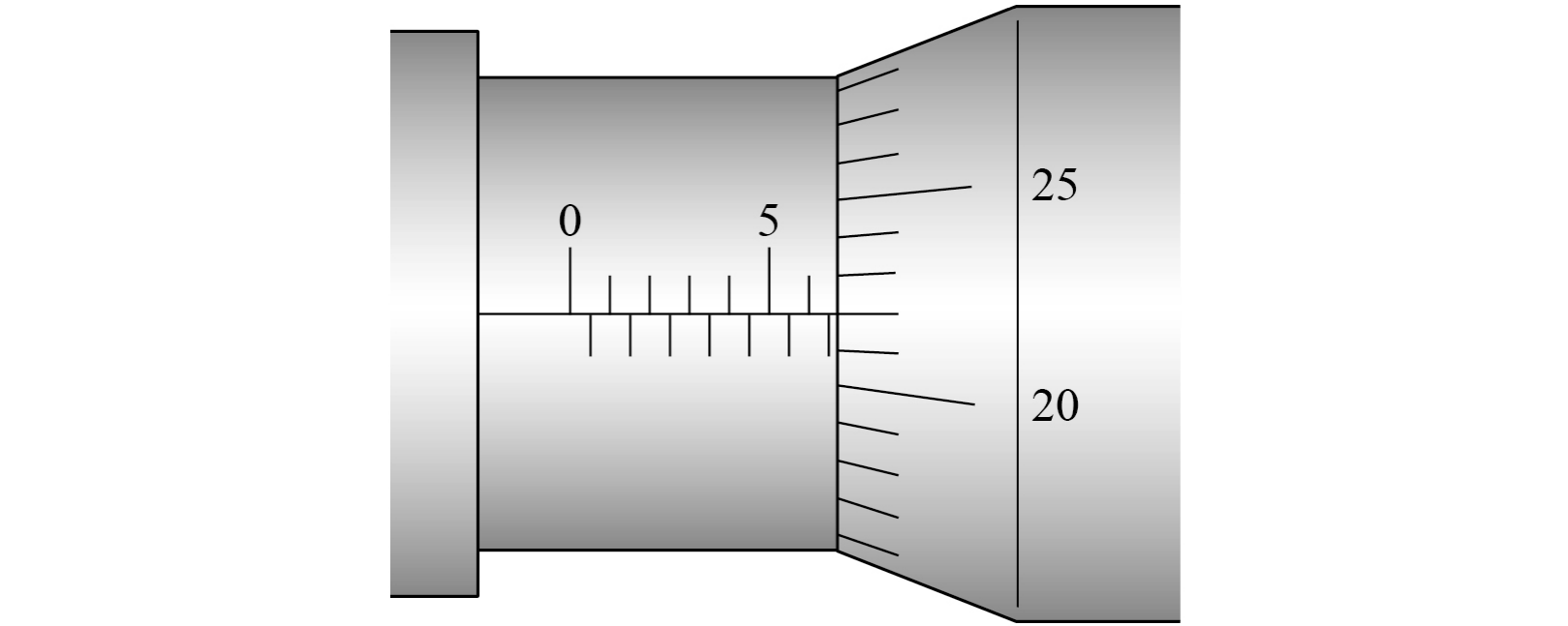
Figure 6 shows the reading on the micrometer.

Figure 6

State the reading on the micrometer.

Describe one procedure the student should use to reduce the uncertainty in the measurement of $y$.

It can be shown that the relationship between $T$ and $M$ is

$T^2=\frac{8{\mathrm{\pi }}^2{L}^{3}M}{Ex{y}^3}$

where $E$ is the Young modulus of the metal.

A student is asked to test the relationship between $T$ and $M$ using the arrangement shown in Figure 5 with the following restrictions:

• $L$ must be kept constant

• $M$ must be made using 20 g, 50 g, and 100 g masses

• the experimental procedure must involve only one independent variable

• a graphical method must be used to obtain a result for $E$

Explain what the student must do to determine $E$.

A different student is asked to use the apparatus in Figure 5 to test the relationship $T^2=k{L}^3$, where $k=\frac{6.9\times {10}^5}{E}$.

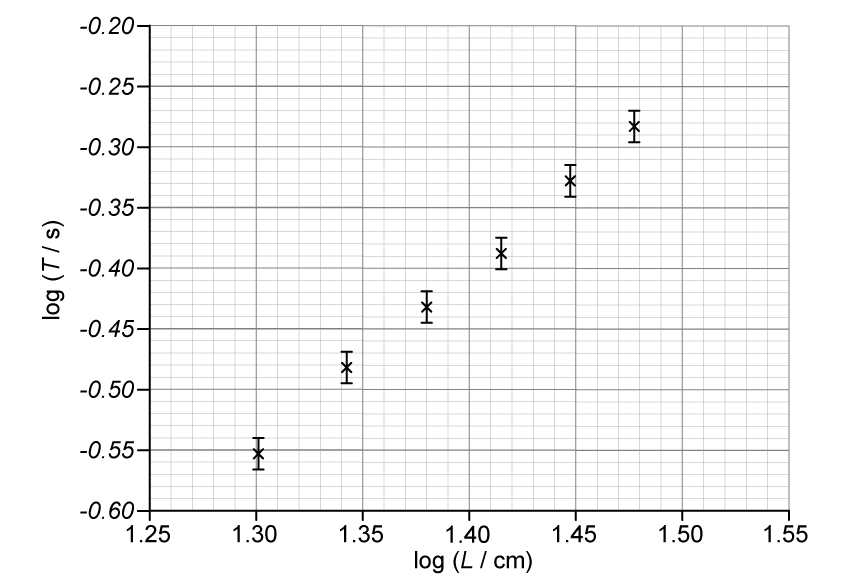
The student plots the graph shown in Figure 7.

The student estimates the percentage uncertainty in each value of $T$ to be 3% and adds error bars to the graph.

Figure 7

Add to the graph in Figure 7

• a line of best fit

• a line of worst fit

Show that the percentage uncertainty in the gradient is about 11%.

Explain how the gradient of the line of best fit confirms that $T^2$ is proportional to $L^3$.

Determine a value for $E$ using Figure 7.

Explain why the percentage uncertainty in $E$ determined from Figure 7 would be very large.

Suggest one change to the experiment that would reduce the percentage uncertainty in $E$.

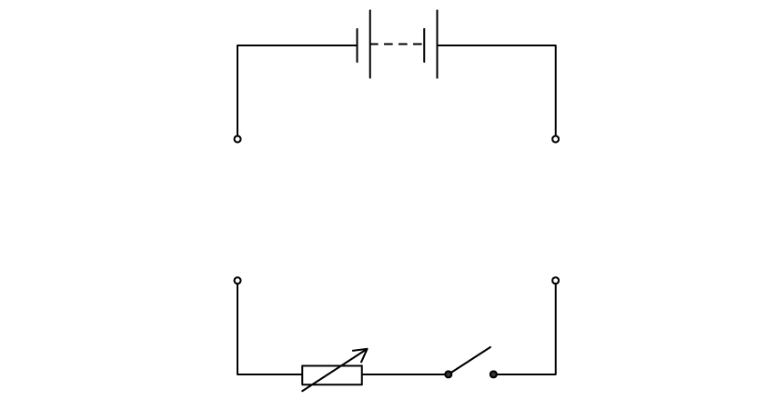
This question is about an investigation into how the terminal potential difference (pd) $V$ across a battery varies with the current $I$ (required practical activity 6).

Figure 8 shows a partially completed circuit diagram for this investigation.

Figure 8

Complete Figure 8 to show how an ammeter and a voltmeter should be connected to measure $I$ and $V$.

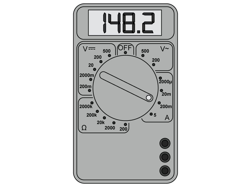
The student uses a multimeter to measure $I$ and $V$.

Figure 9 shows the multimeter set to the 200 mA d.c. current range.

Figure 9

What is the reading on the multimeter?

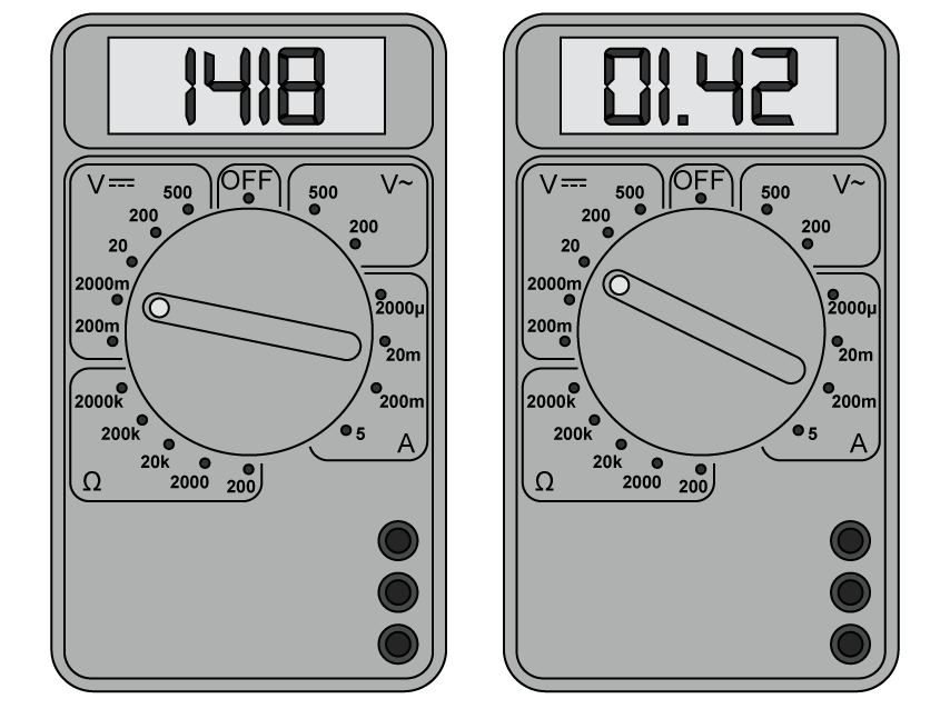
Figure 10 shows how the multimeter displays the value of $V$ when set to two different d.c. voltage ranges.

Figure 10

Explain whether the 2000 mV range or the 20 V range should be used to measure $V$.

Explain why the switch should be opened between readings.

Describe the procedure the student should use to obtain a set of readings of $I$ and $V$.

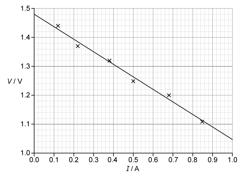
Figure 11 shows a graph of the experimental data.

Figure 11

Determine from Figure 11:

• the emf $\epsilon$ of the battery

• the internal resistance $r$ of the battery.

Determine the percentage uncertainty in $r$ using the multimeter readings from Figure 9 and Figure 10 and the value of $ϵ$ from (f).

The uncertainty in $ϵ$ is negligible.

The battery is made up of two identical cells. The student removes one of the cells from the circuit in Figure 8 and repeats the experiment.

Compare the graph produced for this second investigation with the graph shown in Figure 11.