Components of Aggregate Demand: Consumption & Saving (Cambridge (CIE) A Level Economics): Revision Note

Bridge from AS Level

At AS Level the components of AD were introduced as the identity AD = C + I + G + (X − M), with determinants listed but not explored in technical depth

At A Level, each component is modelled more formally

Consumption and saving are split into autonomous and induced parts and written as functions of income

Autonomous versus induced expenditure

• A key distinction is between autonomous and induced spending:

  • Autonomous spending is independent of the current level of national income

    • It occurs even when Y = 0 and is driven by factors outside the income-expenditure model (interest rates, expectations, government policy)

  • Induced spending varies directly with national income

    • As Y rises, induced spending rises in proportion

• Every component of AD can be broken down into these two elements

• The distinction matters because only induced spending feeds back into the multiplier process, while autonomous spending is the initial injection that the multiplier acts upon

The consumption function

• The consumption function expresses total consumer expenditure as the sum of an autonomous component and an induced component:

C = a + bY

• Where:

  • a = autonomous consumption - the amount consumers spend when Y = 0, financed by dissaving, borrowing or running down wealth

  • b = the marginal propensity to consume (MPC) - the fraction of each additional £1 of income spent on consumption

  • bY = induced consumption - rises as income rises

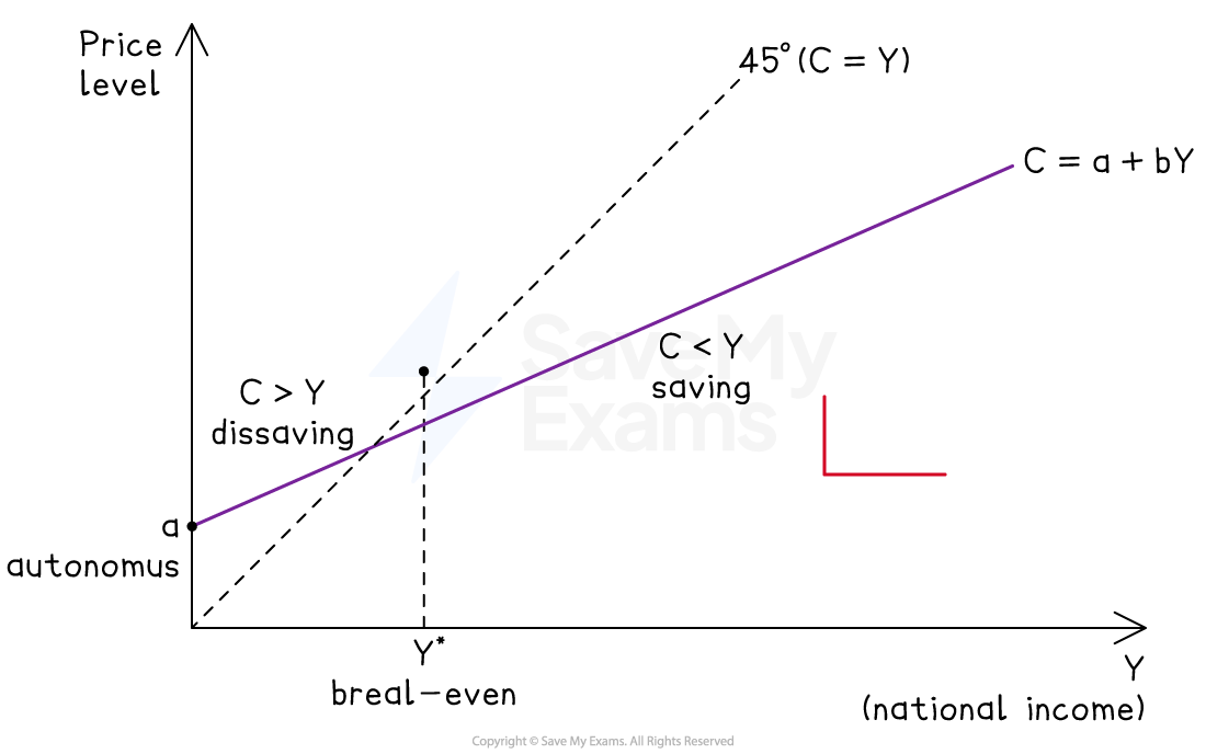
Diagram analysis

• The consumption function starts at a positive vertical intercept a, showing that consumption is positive even when income is zero (autonomous consumption financed by dissaving or borrowing)

• The function slopes upward with gradient b (the MPC), which is positive and less than 1 - each additional £1 of income raises consumption by less than £1

• The 45° line shows every point at which C = Y

• The consumption function crosses the 45° line at the break-even level of income Y*, where consumption exactly equals income and saving is zero

  • To the left of Y*, the function sits above the 45° line - households consume more than their income and must dissave

  • To the right of Y*, the function sits below the 45° line - households consume less than their income and save the remainder

Determinants of autonomous consumption (shifts in the function)

• Autonomous consumption changes when:

  • Wealth rises or falls (the wealth effect - a rise in house or asset prices raises a)

  • Consumer confidence shifts (optimism about future incomes raises a)

  • Interest rates change (lower rates make saving less attractive and borrowing cheaper, raising a)

  • Availability of credit expands or contracts

Determinants of the MPC (slope of the function)

• The slope b depends on:

  • Income distribution - lower-income households have a higher MPC than higher-income households, so redistribution towards the poor raises the aggregate MPC

  • Expectations about future income - if income rises are seen as permanent, MPC is higher than if they are seen as temporary

• The consumption function is central to the multiplier

  • The larger b, the smaller the leakage into saving and the larger the multiplier k = 1 ÷ (1 − b) in a closed economy with no government

The savings function

• Saving is simply the residual of disposable income not spent on consumption. Because Y = C + S by definition in a closed economy with no government:

S = −a + (1 − b)Y or S = −a + sY

• where s = 1 − b is the marginal propensity to save (MPS).

  • Autonomous saving is negative (−a) - at Y = 0 households are dissaving to finance autonomous consumption

  • Induced saving (sY) rises with income - higher income means a larger absolute amount saved even at a constant MPS

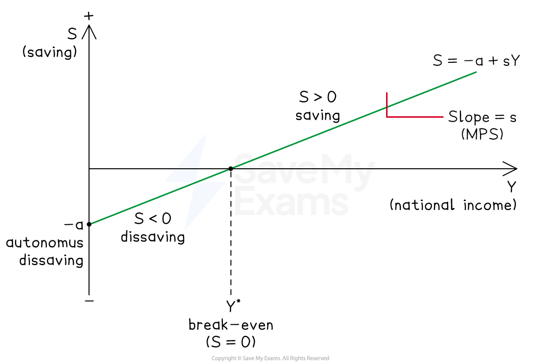
Diagram analysis

• The savings function starts at a negative vertical intercept −a, showing that saving is negative when income is zero (households dissave to finance autonomous consumption)

• The function slopes upward with gradient s (the MPS), positive and less than 1 - each additional £1 of income adds less than £1 to saving

• The function crosses the horizontal axis at the break-even level of income Y*, where saving is zero

  • To the left of Y*, saving is negative (dissaving)

  • To the right of Y*, saving is positive and rises with income

• The savings function is the mirror image of the consumption function: the two must sum to Y at every level of income. Any shift in the consumption function produces an equal and opposite shift in the savings function

Determinants of saving

• The savings function shifts when:

  • Interest rates rise (raising the reward for saving, shifting S up)

  • Confidence falls (precautionary saving rises, shifting S up)

  • Demographic structure changes (ageing populations save differently from younger ones)

  • Tax treatment of savings changes (tax-advantaged savings accounts raise S)

The mirror-image relationship

• Because Y = C + S at every level of income, the consumption function and the savings function are mirror images of one another

  • Any shift in one produces an equal and opposite shift in the other, and both functions share the same break-even level of income Y*

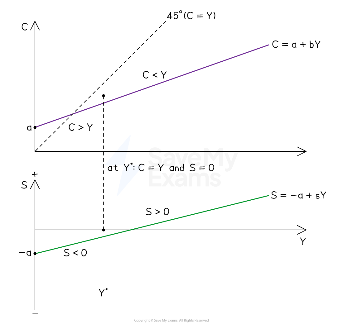
Diagram analysis

• The upper panel shows the consumption function; the lower panel shows the savings function; both share the same horizontal income axis

• At Y = 0, C = a (positive autonomous consumption) and S = −a (equal and opposite autonomous dissaving) - the two intercepts mirror one another

• At Y*, the consumption function crosses the 45° line and the savings function crosses the horizontal axis simultaneously - this is the single break-even level of income at which C = Y and S = 0

  • To the left of Y*: C > Y in the upper panel corresponds to S < 0 in the lower panel (dissaving finances the excess consumption)

  • To the right of Y*: C < Y in the upper panel corresponds to S > 0 in the lower panel (income exceeds consumption, producing positive saving)

• A rise in autonomous consumption (shift of C upward) must be matched by a fall in autonomous saving (shift of S downward) by the same amount