The Effect of the Multiplier on National Income (Cambridge (CIE) A Level Economics): Revision Note

National income determination with the multiplier process

• You are required to understand two complementary approaches for showing the multiplier's effect on national income:

  • The income-expenditure approach (Keynesian 45-degree diagram) - shows why the change in income is a multiple of the initial injection

  • The AD/AS approach - shows what that multiplied change means for real output, the price level and employment

Income-expenditure (45-degree) approach

• This diagram plots:

  • National income (Y) on the horizontal axis

  • Aggregate expenditure (AE = C + I + G + (X − M)) on the vertical axis

  • A 45-degree reference line where Y = AE, representing every possible point at which total planned spending equals total output

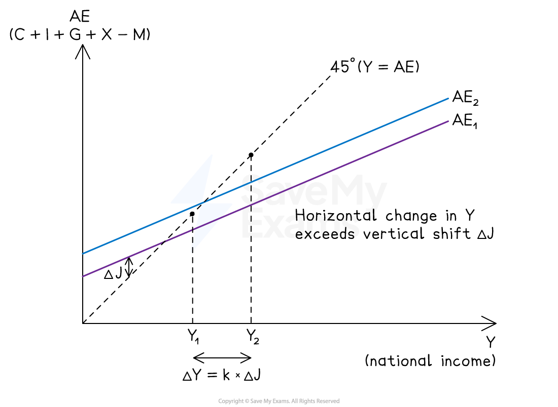
Diagram analysis

• Equilibrium national income occurs at Y₁, where the AE curve crosses the 45-degree line

  • At this point, planned expenditure equals output and there is no pressure for income to change

• A rise in any injection (investment, government spending or exports) shifts the AE curve vertically upward by the size of the injection, ΔJ

  • The new equilibrium forms at Y₂, further along the 45-degree line

  • The horizontal change in income (ΔY) is larger than the vertical shift (ΔJ) because each round of additional spending creates further rounds of income

  • The ratio ΔY ÷ ΔJ is the multiplier k

  • Provided spare capacity exists, firms raise output from Y₁ to Y₂ and employment rises

• This is the graphical form of ΔY = k × ΔJ, and shows the multiplier mechanism most directly - the vertical shift is the cause, the horizontal change is the multiplied effect

AD/AS approach

• The same multiplier process can be shown on an AD/AS diagram, using two successive rightward shifts of AD

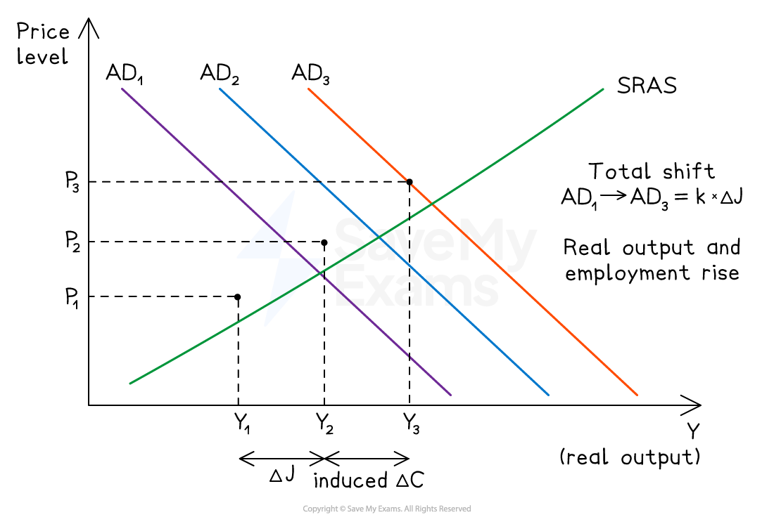
Diagram analysis

• Initial equilibrium is at P₁Y₁, where AD₁ intersects SRAS

• The initial injection shifts AD from AD₁ to AD₂, a rightward shift equal to ΔJ

• The multiplier process then plays out through successive rounds of induced consumer spending, shifting AD further right from AD₂ to AD₃

  • The total horizontal shift from AD₁ to AD₃ equals k × ΔJ - the multiplied change in national income

  • At the new equilibrium P₃Y₃, real output is higher, employment has risen as firms expand to meet demand, and the price level has risen

• The balance of output versus price effects depends on the slope of SRAS: with significant spare capacity, the gain is mostly in real output and employment

  • near full capacity most of the effect becomes inflationary with limited employment gains

Calculating the effect of changing AD on national income

• Any change in a component of aggregate demand (C, I, G or X − M) feeds through the multiplier to produce a larger change in national income. The core calculation is:

ΔY = k × ΔJ

Evaluation and limitations

• The multiplier is a powerful tool but rests on the following strong assumptions:

  • Assumes a stable MPC - in reality, MPC varies with income level, confidence and the phase of the economic cycle

  • Assumes spare capacity - if the economy is at or near full employment, the multiplied increase in AD translates into inflation rather than output growth

  • Ignores time lags - the full multiplier effect takes several quarters to work through; it is not instantaneous

  • Ignores crowding out - if the initial injection is government spending financed by borrowing, higher interest rates may reduce private investment, partially offsetting the multiplier

  • Small open economies have small multipliers - countries like Singapore or Ireland have very high MPMs, so domestic multipliers are close to 1; fiscal stimulus leaks abroad

  • The reverse multiplier amplifies downturns - a fall in exports or investment reduces national income by a multiple of the initial fall, which is why recessions deepen rapidly

Why do multiplier estimates vary internationally

• IMF estimates of fiscal multipliers typically range from 0.5 to 2.5 depending on country and conditions. Multipliers tend to be larger in:

  • Large economies with low import dependence (e.g. the USA)

  • Economies in recession with significant spare capacity

  • Economies where monetary policy does not offset fiscal expansion

• Multipliers tend to be smaller in:

  • Small, highly open economies (Singapore, the Netherlands)

  • Economies at or near full employment

  • Economies with high public debt where consumers save extra income in anticipation of future tax rises (Ricardian equivalence)

• This variation is why blanket claims about fiscal policy effectiveness are rarely correct - the multiplier is context-dependent