Causes & Effects of Changing Exchange Rates (Cambridge (CIE) A Level Economics): Revision Note
Exam code: 9708

Changes in the exchange rate under different systems
Changes under a floating system
Under a freely floating exchange rate, the rate changes continuously in response to:
Interest rate differentials
Higher domestic interest rates attract capital inflows (hot money), increasing demand for the currency and causing appreciation
Inflation differentials
Higher domestic inflation makes exports less competitive, reducing export demand and causing depreciation; this is the basis of purchasing power parity (PPP) theory
Current account movements
A current account deficit means more domestic currency is being sold to buy foreign goods and services, putting downward pressure on the rate
Speculation
If traders expect a currency to fall, they sell it now, creating a self-fulfilling depreciation; conversely, expected appreciation attracts speculative buying
Economic performance and confidence
Strong growth and political stability attract FDI and portfolio investment, increasing currency demand
Changes under a fixed system
The exchange rate does not change as a result of market forces - the central bank neutralises market pressure through intervention
The rate can only change through a deliberate policy decision (devaluation or revaluation)
If market pressure against the peg becomes overwhelming - for example, if a current account deficit persists and reserves are depleted - the peg may be forced to collapse, as occurred in the 1992 ERM crisis when sterling was forced out of the European Exchange Rate Mechanism
Changes under a managed float
The rate moves with market forces within informal limits
The central bank intervenes to 'lean against the wind' - selling the currency if it rises too far, buying if it falls too far
The rate can trend in one direction over time if fundamentals support it, unlike a strict fixed rate
The Marshall-Lerner Condition and J-Curve
The Marshall-Lerner condition states that a currency depreciation will improve the current account only if the sum of the price elasticities of demand for exports and imports exceeds one
PED(X) + PED(M) > 1
When the condition is satisfied, the volume response to the price change is large enough to outweigh the adverse initial price effect, and the current account improves
When the condition is not satisfied (PED(X) + PED(M) < 1), demand for both exports and imports is too inelastic — the current account worsens following depreciation
This follows the revenue rule which states that in order to increase revenue, firms should lower prices for products that are price elastic in demand
If the combined elasticity of exports/imports is less than 1 (inelastic), a depreciation (fall in price) will actually worsen the current account balance
The J-Curve effect
It is also important to recognise that there is a time lag between the depreciation of the currency and any subsequent improvement in the current account balance
This time lag is explained by the J-Curve effect
It takes time for firms and consumers to respond to changes in price
Once it becomes evident that price changes will last for a longer period of time, firms and consumers change their patterns
E.g. a firm in the USA has been importing electric scooters from the UK. If the Euro depreciates, the price of scooters in France becomes relatively cheaper. In the short term, the USA firm will not switch immediately to purchasing scooters from France, as the exchange rate may soon bounce back. They also have a positive relationship with their UK suppliers. In the long term they are likely to switch

The J Curve explains what happens to a trade balance over time when the country's currency depreciates
Diagram analysis
In the short run, the sum of PEDs for exports and imports was less than one / inelastic (or the Marshall-Lerner condition was not fulfilled) so the deficit widens
However, in the long run the Marshall-Lerner condition is met so it leads to a surplus
With any currency depreciation/devaluation, the trade balance will initially worsen before it improves
Existing contracts - firms and households are locked into import and export contracts agreed at the old exchange rate; until these expire, trade volumes cannot adjust to the new relative prices
Consumer habits and brand loyalty - buyers do not switch suppliers immediately following a price change; it takes time for consumers and firms to identify cheaper alternatives, trial them and build new supply relationships
Supply-side capacity constraints - domestic export industries cannot instantly scale up production to meet increased foreign demand following depreciation; new capacity takes time to build, meaning export volumes rise only gradually even when export prices have fallen
Case Study
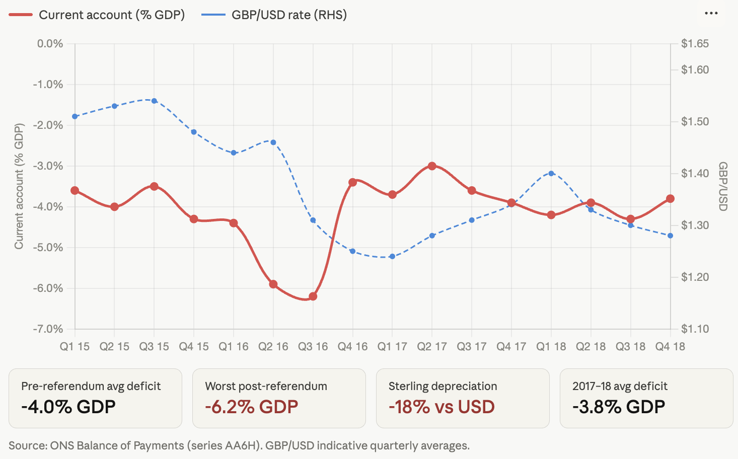
UK current account following the Brexit depreciation, 2016–2018
The context
Following the Brexit referendum in June 2016, sterling depreciated approximately 15% on a trade-weighted basis - one of the largest peacetime depreciations of a major currency in modern history. With the UK running a persistent current account deficit of around 5–6% of GDP, the depreciation provided a near-perfect real-world test of both the Marshall-Lerner condition and the J-curve effect.
Actions taken
Sterling fell from approximately £1 = $1.48 to £1 = $1.22 by January 2017 — an 18% depreciation against the US dollar
The Bank of England cut interest rates and expanded quantitative easing in August 2016, reinforcing the depreciation
The UK remained in the EU single market during transition, meaning trade barriers were unchanged
Outcomes
In the short run the current account deficit widened, consistent with J-curve theory - import costs rose immediately while export volumes were slow to respond due to existing contracts and capacity constraints
UK goods export volumes began rising from mid-2017 as foreign buyers responded to lower sterling prices, consistent with the Marshall-Lerner condition being met in the long run
However, the deficit remained above 3% of GDP through 2018 — suggesting PED for UK exports and imports was relatively inelastic, and that Brexit uncertainty constrained the full Marshall-Lerner improvement
The case illustrates that even when the condition is met, structural factors can limit the scale of current account improvement

Unlock more, it's free!
Join the 100,000+ Students that ❤️ Save My Exams
the (exam) results speak for themselves:

Was this revision note helpful?