AP®MathsCollege BoardPrecalculusStudy GuidesExponential & Logarithmic FunctionsModeling with Exponential & Logarithmic FunctionsLogarithmic Models

Logarithmic Models (College Board AP® Precalculus): Study Guide

Written by: Roger B

Reviewed by: Mark Curtis

Updated on 13 April 2026

Logarithmic models

When is a logarithmic model appropriate?

Logarithmic functions are the inverses of exponential functions
- so they model the 'reverse' type of relationship
An exponential function has
- outputs that change proportionally (multiplicatively)
  - as inputs change additively (by equal amounts)
A logarithmic function has the opposite behavior
- input values change proportionally
  - over equal-length output-value intervals
- In other words, the inputs must be multiplied by a constant factor
  - to produce equal increases in the output
- E.g. the Richter scale for earthquake magnitude is logarithmic
  - Each increase of 1 on the scale corresponds to a tenfold increase in the measured amplitude of the earthquake

How do I construct a logarithmic model from two data points?

A logarithmic model can be constructed from two input-output pairs using the form $f (x) = a + b \ln (x + c)$
- where $c$ is often determined by the context
  - commonly $c = 0$ or $c = 1$
- On the exam, a question typically provides the form of the model
  - e.g. $G (t) = a + b \ln (t + 1)$
  - and asks you to find the constants $a$ and $b$

Here is the general process (using $f (x) = a + b \ln (x + c)$ with data points $(x_{1}, y_{1})$ and $(x_{2}, y_{2})$ )
- Assume that $c$ is known (it is usually given on the exam)
- Substitute each data point into the function to get two equations
  - $y_{1} = a + b \ln (x_{1} + c)$
  - $y_{2} = a + b \ln (x_{2} + c)$
- Solve the system for $a$ and $b$
- Often one of the data points will cause the argument inside one of the logarithms to be equal to 1
  - This simplifies things greatly since $\ln (1) = 0$
  - It gives $a = y_{1}$ directly

Example: A study uses test scores to track academic content retention. At $t = 0$ months, the average score is 75 points. At $t = 3$ months, the average score is 70.84 points. The model to be used is $R (t) = a + b \ln (t + 1)$ .
- $R (0) = 75$ so
  - $75 = a + b \ln (0 + 1) \Rightarrow 75 = a + b \ln (1) \Rightarrow a = 75$
    - this uses $\ln (1) = 0$ in the final step
- And $R (3) = 70.84$ , so
  - $70.84 = a + b \ln (3 + 1) \Rightarrow 70.84 = 75 + b \ln (4)$
    - using the value of $a$ from the previous step
- Solve for $b$
  - $- 4.16 = b \ln (4) \Rightarrow b = - \frac{4.16}{\ln (4)} \approx - 3.001$
- So the model is
  - $R (t) = 75 - 3.001 \ln (t + 1)$

Examiner Tips and Tricks

Constructing a model from two data points tends to appear in a free response question on every exam, so practice this skill thoroughly.

Non-exact values of $a$ and $b$ must be given as decimal approximations correct to three decimal places
- The scoring guidelines are strict about this
You can solve for $a$ and $b$ either algebraically or by using your graphing calculator
- The scoring guidelines note that "supporting work is not required", so using a calculator is perfectly acceptable
Store intermediate values in your calculator rather than rounding them
- Rounding too early can produce final answers that are not accurate to three decimal places

Can a logarithmic model also be constructed from a proportion and a zero?

Yes, a logarithmic model can be constructed from:
- An appropriate proportion
  - i.e. the multiplicative factor for inputs over equal output intervals
- A real zero
  - an input value where the output is zero
This connects to the inverse relationship with exponential functions
- If an exponential function has base $b$ and initial value 1
  - then its inverse logarithmic function has base $b$ and a zero at $x = 1$
E.g. for a model in the form $f (x) = \log_{b} (k x)$
- suppose input values are multiplied by 2 for each increase by 1 in the output
  - and the output is 0 when $x = 4$
- The proportion, which determines the base of the logarithm, is $b = 2$
  - inputs double per unit output increase
- And the zero is at $x = 4$ , so $k x$ must equal 1 when $x = 4$
  - because $\log_{b} (1) = 0$
- Therefore the model is
  - $f (x) = \log_{2} (\frac{x}{4})$

How can transformations be used to build a logarithmic model?

Logarithmic models can be constructed by applying transformations to the base function $f (x) = \log_{b} x$
The transformations allows the function to match the characteristics of the context or data:
- A vertical shift $\log_{b} (x) + k$
  - adds $k$ to all the output values
    - the graph goes through $(1, k)$ instead of $(1, 0)$
    - the location of the zero will move
- A horizontal shift $\log_{b} (x + h)$
  - shifts the graph by $h$ units to the left
    - the zero will occur at $(1 - h, 0)$ instead of at $(1, 0)$
- A vertical dilation $a \log_{b} x$
  - adjusts the rate of growth

How do I construct a logarithmic model using technology?

When data does not fit a simple logarithmic form exactly
- a graphing calculator can fit a logarithmic regression model to the data
This is done using the LnReg (or similar) function on most graphing calculators
- The calculator determines the best-fit values for the constants $a$ and $b$
- in the model $a + b \ln x$

Why is the natural logarithm often used in modeling?

The natural logarithm ( $\ln$ , with base $e \approx 2.718$ ) appears frequently in real-world models
- Many natural processes involve continuous growth or decay
  - and the natural base $e$ arises naturally in these contexts
In logarithmic modeling questions on the exam, $\ln$ appears far more regularly than other logarithm bases

How can a logarithmic model be used to make predictions?

Once a logarithmic model is constructed, it can be used to predict values of the dependent variable
- by substituting input values into the function
You can also predict input values
- by substituting output values into the function
- and solving to find the corresponding input value
Some things to keep in mind:
- Logarithmic functions grow very slowly for large inputs
  - Predictions for very large input values may not change much
- The model may not remain valid beyond the range of data used to construct it
  - Just as with any model

Worked Example

The number of bird species observed in a nature reserve can be modeled by the function $S$ given by $S (t) = a + b \ln (t + 1)$ , where $S (t)$ is the total number of species observed during the first $t$ months of a long-term survey.

At the start of the survey $(t = 0)$ , 15 species were observed. After 5 months $(t = 5)$ , 24 species had been observed.

(a) Use the given data to write two equations that can be used to find the values for constants $a$ and $b$ in the expression for $S (t)$ .

Answer:

Substitute the two data points into $S (t) = a + b \ln (t + 1)$

$S (0) = 15$
$a + b \ln (0 + 1) = 15$

$a + b \ln (1) = 15$

$S (5) = 24$
$a + b \ln (5 + 1) = 24$

$a + b \ln (6) = 24$

(b) Find the values for $a$ and $b$ as decimal approximations.

Answer:

Use $\ln (1) = 0$ in the first equation

$a = 15$

Substitute that into the second equation

$15 + b \ln (6) = 24$

$b \ln (6) = 9$

$b = \frac{9}{\ln 6} = 5.022995 . . .$

Round to 3 decimal places

$b = 5.023 (3 d . p .)$

Worked Example

Two function models $f$ and $g$ are constructed to represent the depth of water, in meters, in a reservoir after $t$ weeks, for $t \geq 2$ . The functions are given by $f (t) = 16 - 3.6 \ln t$ and $g (t) = - t + 16$ .

What is the first time $t$ that the depth predicted by the logarithmic model will be 0.1 meters more than the depth predicted by the linear model?

(A) $t = 8.713$

(B) $t = 7.213$

(D) $t = 5.713$

Answer:

You need to find when $f (t) - g (t) = 0.1$

$(16 - 3.6 \ln t) - (- t + 16) = 0.1$

$t - 3.6 \ln t = 0.1$

This equation cannot be solved algebraically, so use a graphing calculator

Graph $y_{1} = t - 3.6 \ln t$ and $y_{2} = 0.1$
- then find the intersection (or solve $t - 3.6 \ln t - 0.1 = 0$ ).
The $t$ -value of the intersection is the time you are looking for

Be careful here, as there are actually 2 points of intersection

But only one of them occurs for the interval $t \geq 2$

Graph of a curve intersecting y=0.1 at labelled point (7.21337, 0.1), on a grid with marked axes.

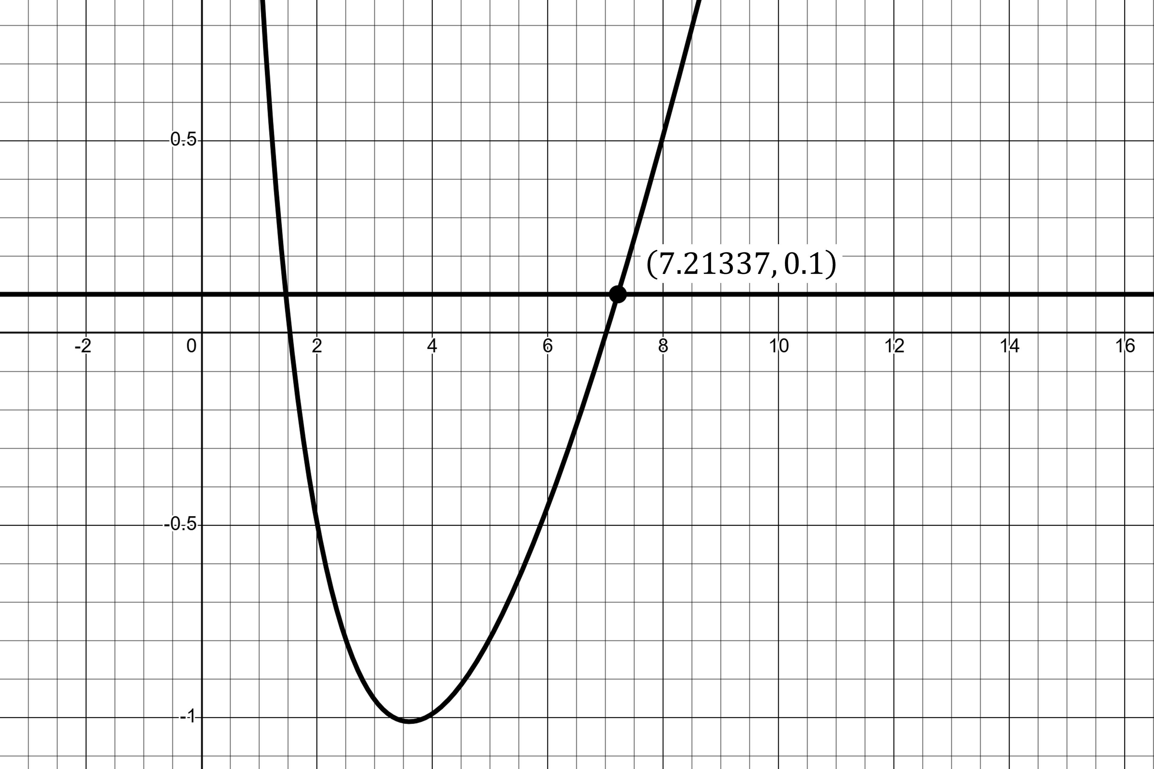
To 3 decimal places that $t$ -coordinate has value 7.213

(B) $t = 7.213$

Examiner Tips and Tricks

The second Worked Example requires using your graphing calculator because the equation mixes a polynomial term ( $t$ ) with a logarithmic term ( $\ln t$ ).

Recognizing when technology is needed (rather than spending time trying to solve algebraically) is an important exam skill

Also note that you may also be able to solve $t - 3.6 \ln t = 0.1$ using your calculator's equation solving functionality.

This is an alternative to drawing a graph and finding the intersection
You would still need to take care to find the solution that satisfies $t \geq 2$

Unlock more, it's free!

Join the 100,000+ Students that ❤️ Save My Exams

the (exam) results speak for themselves:

I would just like to say a massive thank you for putting together such a brilliant, easy to use website.I really think using this site helped me secure my top gradesin science and maths. You really did save my exams! Thank you.

Beth
IGCSE Student

This website is soooo useful and I can’t ever thank you enough for organising questions by topic like this. Furthermore, the name of the website could not have been more appropriate as it literally did SAVE MY EXAMS!

Fathima
A Level Student

Incredible! SO worth my money, the revision notes have everything I need to know and are so easy to understand. I actually enjoy revising! It makes me feel a lot more confident for my GCSEs in a few months.

Kate
GCSE Student

Absolutely brilliant, both my girls used it for A levels and GCSE. It's saves on paper copies, also beneficial exam questions ranked from easy to hard. It's removed a lot of stress from the exams.

Sameera
Parent

Just to say that your resources are the best I have seen and I have been teaching chemistry at different levels for about 40 years

Mark
Chemistry Teacher

Excellent

Logarithmic Models (College Board AP® Precalculus): Study Guide

Logarithmic models

When is a logarithmic model appropriate?

How do I construct a logarithmic model from two data points?

Examiner Tips and Tricks

Can a logarithmic model also be constructed from a proportion and a zero?

How can transformations be used to build a logarithmic model?

How do I construct a logarithmic model using technology?

Why is the natural logarithm often used in modeling?

How can a logarithmic model be used to make predictions?

Worked Example

Worked Example

Examiner Tips and Tricks

Unlock more, it's free!

Join the 100,000+ Students that ❤️ Save My Exams

Author: Roger B

Reviewer: Mark Curtis