Required Practical: Investigating Magnetic Fields in Wires (AQA A Level Physics): Revision Note
Exam code: 7408

Required practical: investigating magnetic fields in wires
Aim of the experiment
The overall aim of this experiment is to calculate the magnetic flux density of a magnet
This is done by measuring the force on a current-carrying wire placed perpendicular to the field
This is just one example of how this required practical might be carried out
Variables
Independent variable = Current,
Dependent variable = mass,
Control variables:
Length of wire,
Magnetic Flux density,
E.m.f. of the power supply
Equipment list
Apparatus | Purpose |
|---|---|
Electronic top-pan balance | To measure the mass |
Thick copper wire | The object which will experience the magnetic force |
Variable resistor | To vary the current flowing through the wire |
DC power supply | To provide the potential difference through the wire |
Ammeter | To measure the current through the wire |
Two magnets with opposite poles in a metal cradle | To create the magnetic field |
Clamp (retort) stand | To hold the wire in the magnetic field |
30 cm ruler | To measure the length of the magnet (which will count as the length of the wire) |
Crocodile clips | To hold both ends of the wire in place on the clamp stand |
Resolution of measuring equipment:
Ammeter = 0.01 A
Variable resistor = 0.01 Ω
Top-pan balance = 0.01 g
Ruler = 1 mm
Method
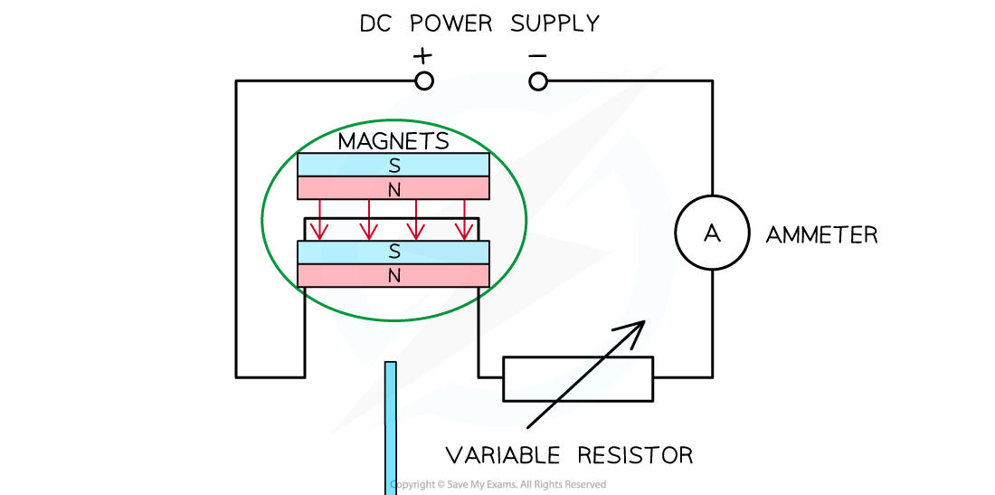
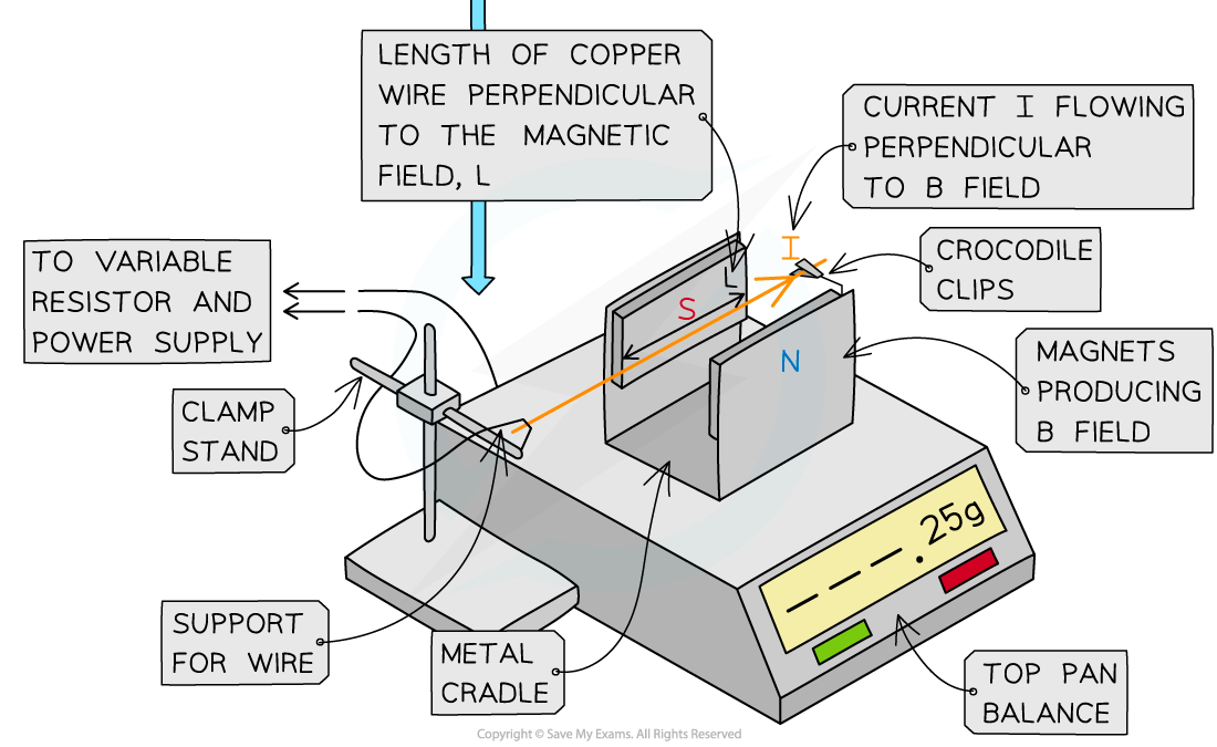
Set up the apparatus as shown above. Make sure the wire is completely perpendicular in between the magnets.
Measure the length of one of the magnets using the 30 cm ruler. This will be the length of the wire in the magnetic field.
Once the magnet is placed on the top-pan balance, and whilst there is no current in the wire, reset the top-pan balance to 0 g.
Adjust the resistance of the variable resistor so that a current of 0.5 A flows through the wire as measured on the ammeter.
The wire will experience a force upwards. Due to Newton’s third law, the force pushing downwards will be the mass on the balance. This movement will be very small, so it may not be completely visible.
Record the mass on the top-pan balance from this current.
Repeat the procedure by increasing the current in intervals of 0.5 A between eight to ten readings for the current (not exceeding 6 A).
Repeat the experiment at least three times, and calculate the mean of the mass readings.
An example table might look like this:
Current / A | Mass / g | Mass / g | Mass / g | Average mass / g |
|---|---|---|---|---|
0.50 | ||||
1.00 | ||||
1.50 | ||||
2.00 | ||||
2.50 | ||||
3.00 | ||||
3.50 | ||||
4.00 | ||||
4.50 | ||||
5.00 |
Analysing the results
The magnetic force on the wire is:
Where:
= magnetic force (N)
= magnetic flux density (T)
= current (A)
= length of the wire (m)
Since where is the mass in kilograms, equating these gives:
Rearranging for mass :
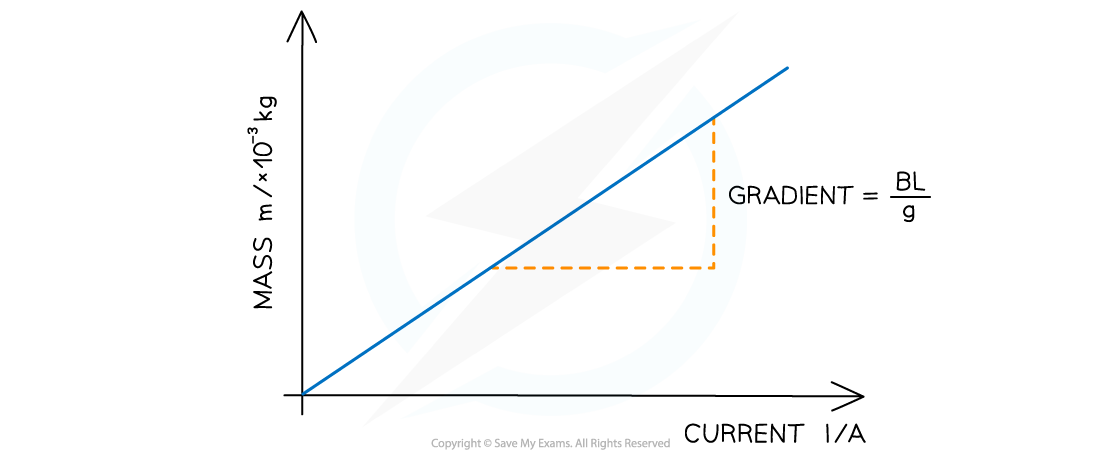
Comparing this to the straight-line equation:
(mass)
(current)
Gradient,
y-intercept, c = 0
Plot a graph of against and draw a line of best fit
Calculate the gradient
The magnetic flux density is:
Evaluating the experiment
Systematic Errors:
Make sure top-pan balance starts at 0 to avoid a zero error
Random Errors:
Repeat the experiment by turning the magnet in the metal cradle and the wire by 90º
Make sure no high currents (up to 6 A) pass through the copper wire, otherwise, the wire’s resistance will increase and affect the experiment
Safety considerations
Keep water or any fluids away from the electrical equipment
Make sure no wires or connections are damaged and contain appropriate fuses to avoid a short circuit or a fire
High currents through the wire will cause it to heat up
Make sure not to touch the wire when current is flowing through it
Worked Example
A student investigates the relationship between the current and the mass measured on a top-pan balance due to the magnetic force on a current-carrying wire. They obtain the following results:
Current / A | Mass / | Mass / | Mass / |
|---|---|---|---|
0.50 | 0.10 | 0.11 | 0.11 |
1.00 | 0.22 | 0.23 | 0.22 |
1.50 | 0.34 | 0.35 | 0.33 |
2.00 | 0.43 | 0.43 | 0.43 |
2.50 | 0.56 | 0.57 | 0.57 |
3.00 | 0.64 | 0.66 | 0.68 |
3.50 | 0.76 | 0.77 | 0.78 |
4.00 | 0.87 | 0.86 | 0.86 |
4.50 | 0.99 | 1.00 | 0.99 |
5.00 | 1.10 | 1.10 | 1.09 |
The mean length of the wire in the magnetic field was found to be 0.05 m.
Using the data in the table, calculate the magnetic flux density.
[4]
Answer:
Step 1: Complete the table
Add an extra column ‘Average mass / × 10-3 kg’ and calculate this for each mass
Current / A | Mass / | Mass / | Mass / | Average mass / |
|---|---|---|---|---|
0.50 | 0.10 | 0.11 | 0.11 | 0.11 |
1.00 | 0.22 | 0.23 | 0.22 | 0.22 |
1.50 | 0.34 | 0.35 | 0.33 | 0.34 |
2.00 | 0.43 | 0.43 | 0.43 | 0.43 |
2.50 | 0.56 | 0.57 | 0.57 | 0.57 |
3.00 | 0.64 | 0.66 | 0.68 | 0.66 |
3.50 | 0.76 | 0.77 | 0.78 | 0.77 |
4.00 | 0.87 | 0.86 | 0.86 | 0.86 |
4.50 | 0.99 | 1.00 | 0.99 | 0.99 |
5.00 | 1.10 | 1.10 | 1.09 | 1.10 |
[1 mark]
Step 2: Plot the graph of average mass against current
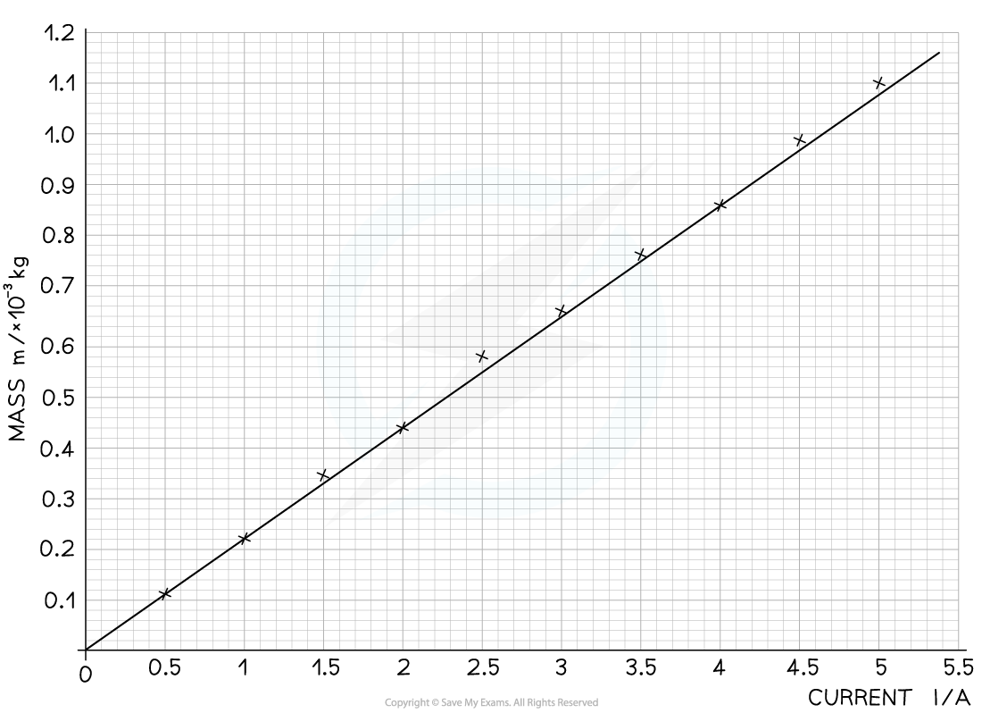
Make sure the axes are properly labelled and the line of best fit is drawn with a ruler [1 mark]
Step 3: Calculate the gradient of the graph
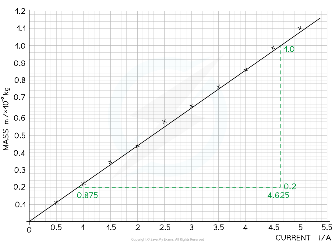
The gradient is calculated using:
[1 mark]
Step 4: Calculate the magnetic flux density
[1 mark]

Unlock more, it's free!
Join the 100,000+ Students that ❤️ Save My Exams
the (exam) results speak for themselves:

Was this revision note helpful?
Build on this topic